How It Works: Trapezoid Integration

How It Works : Integrate by the Trapezoid Rule

In related post I used a numerical integration function from Bahder, Mathematica for Scientists and Engineers, to integrate a sawtooth function. This is a great book. Despite having been written in 1995, it's a wealth of 'under the hood' insights into the Wolfram Language. Here is a second function from Bahder for integration via the trapezoid rule that is more sophisticated than the first one. And due to using built-in Listable functionality in Dot and Plus it's about twice as fast

The syntax of the parameter uses a named Pattern to check the data parameter to see if it is a List of 2-element (x,y) pairs, then uses Condition to make sure that data contains more than one point.

Here is the formula for integration by the trapezoid rule:

And here is Bahder's code. The syntax of the parameter uses a named Pattern to check data to see if it is a List of 2-element (x,y) pairs, then uses Condition to make sure that data contains more than one point.

Clear@integrateTrapezoid;
integrateTrapezoid[data:{{_,_}..}/;Length@data>1]:=Module[{xDifferences,ySums},
xDifferences=Dot[{-1,1},#]&/@Partition[First/@data,2,1];
ySums=Apply[Plus,Partition[Last/@data,2,1],{1}];
Plus@@(xDifferences,ySums)/2
]

The Dot product multiplies each vector (List) term by term and sums them.

Dot[{a,b,c},{x,y,z}]

a x+b y+c z

Let's check to make sure the abbreviated operators for Apply and Divide will work as intended; which they will. Apply is 'stickier' than Divide and so Plus will be evaluated before taking the average (dividing by 2).

Precedence/@{Apply,Divide}

{620.,470.}

We test it on his data and.. it doesn't work. There is a bug.

data1={{1.2,51.3},{2.3,72.8},{3.0,87.1},{3.7,53.2}};

integrateTrapezoid@data1

{62.6,80.3,70.5}

Let's add some Print statements, which suffice for debugging all pure functional programs, that is, short ones.

Clear@integrateTrapezoid;integrateTrapezoid[data:{{_,_}..}/;Length@data>1]:=Module[{xDifferences,ySums},
xDifferences=Dot[{-1,1},#]&/@Partition[First/@data,2,1];
Print@xDifferences;
ySums=Apply[Plus,Partition[Last/@data,2,1],{1}];
Print@ySums;
Plus@@(xDifferences,ySums)/2
]

With the Print statement results it's easy to see that xDifferences is indeed the difference between successive x-points and ySums is the sum of each pair of successive y-values.

integrateTrapezoid@data1

{1.1,0.7,0.7}
{124.1,159.9,140.3}
{62.6,80.3,70.5}

I see the bug. We should be multiplying xDifferences by ySums, not listing them. There's a lesson: Always use a multiplication symbol in code rather than a space, which might be mis-read as I did in Bahder's code. We'll add the multiplication and remove the Print statements.

Clear@integrateTrapezoid;integrateTrapezoid[data:{{_,_}..}/;Length@data>1]:=Module[{xDifferences,ySums},
xDifferences=Dot[{-1,1},#]&/@Partition[First/@data,2,1];
ySums=Apply[Plus,Partition[Last/@data,2,1],{1}];
Print@(xDifferences*ySums);
Plus@@(xDifferences*ySums)/2
]

Now we get the correct answer.

integrateTrapezoid@data1

{136.51,111.93,98.21}
173.325

Let's try it on something else.

data2={{0.0,0.0},{1.0,1.0},{2.0,0.0},{3.0,2.0},{4.0,0.0},{5.0,2.0},{6.0,1.0},{7.0,3.0},{8.0,0.0},{9.0,2.0},{10.0,0.0}};
Graphics[Line@data2,Axes->True]

integrateTrapezoid@data2

{1.,1.,2.,2.,2.,3.,4.,3.,2.,2.}
11.

Trusting we got xDifferences and ySums right, we can copy and paste them into the program final line by hand to double-check its validity.

Plus@@{1.`,1.`,2.`,2.`,2.`,3.`,4.`,3.`,2.`,2.`}/2

11.

Recommended:

Compiling a Function: Mandelbrot Set

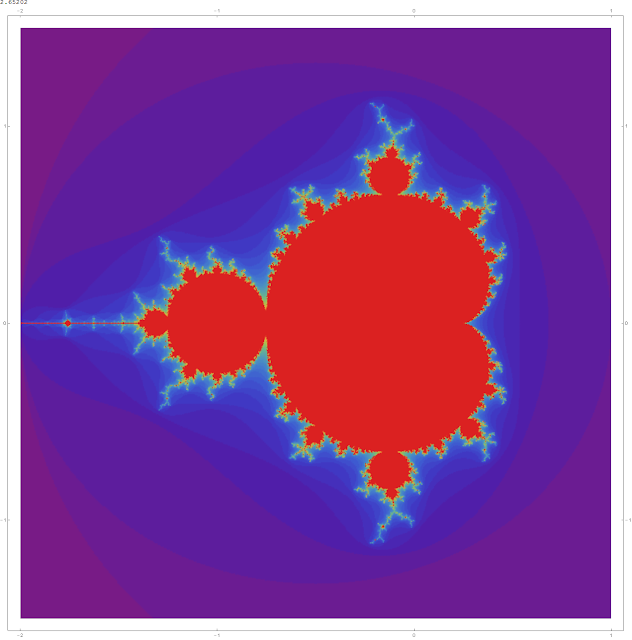
Computing the Mandelbrot set is a classic example of the need to Compile a Mathematica function (see Ruskeepää, p. 451). You just need to get the syntax right for a successful Compile. Below, the first argument is the parameter, c, and its type, Complex. The entire Module is the second argument, the expression to be compiled. Definitely try this at home!

Clear@mandelbrot;mandelbrot=Compile[{{c,_Complex}},Module[{z=0+0I,n=0},While [Abs@z<2&&n<50,z=z^2+c;n++];n  ] ]

CompiledFunction[Argument count: 1
Argument types: {_Complex}

The CompiledFunction can be applied to individual numbers. The criteria for inclusion in the Mandelbrot set is, after a limited number of iterations of z = z^2 + c (in this case 50), is its absolute value less than a given number (in this case 2). The absolute value of a complex number is its Euclidean distance from the origin. If the absolute value of a number exceeds 2 before 50 iterations, e.g. 4, it is excluded.

mandelbrot[0.2+I]

4

mandelbrot[0.2+0.2I]

50

Let's do some heavy-duty computing. As a precaution we'll increase the RAM allocated to Mathematica.

Needs@"JLink`";
ReinstallJava[JVMArguments->"-Xmx6000m"]

LinkObject[[]

Start with a couple of individual plots. I use ImageSize->Full so when you do this yourself a large image will automatically be generated. On my Dell Optiplex 900 these take 2.68 seconds each.

Timing[DensityPlot[mandelbrot[x+I y],{x,-2,1},{y,-1.5,1.5},ColorFunction->Hue,PlotPoints->200,Mesh->False,ImageSize->Full,FrameTicks->{{-2,-1,0,1},{-1,0,1}}]]//Column

 Timing[DensityPlot[mandelbrot[x+I y],{x,-2,1},{y,-1.5,1.5},ColorFunction->"Rainbow",PlotPoints->200,Mesh->False,ImageSize->Full,FrameTicks->{{-2,-1,0,1},{-1,0,1}}]]//Column

 I'm kind of curious about all the built-in ColorFunctions. Let's plot Mandelbrot sets using each of them. Here they are. I reverse the order since I like some of the ones at the end best.

colorFunctions=ColorData@"Gradients"

{AlpineColors,Aquamarine,ArmyColors,AtlanticColors,AuroraColors,AvocadoColors,BeachColors,BlueGreenYellow,BrassTones,BrightBands,BrownCyanTones,CandyColors,CherryTones,CMYKColors,CoffeeTones,DarkBands,DarkRainbow,DarkTerrain,DeepSeaColors,FallColors,FruitPunchColors,FuchsiaTones,GrayTones,GrayYellowTones,GreenBrownTerrain,GreenPinkTones,IslandColors,LakeColors,LightTemperatureMap,LightTerrain,MintColors,NeonColors,Pastel,PearlColors,PigeonTones,PlumColors,Rainbow,RedBlueTones,RedGreenSplit,RoseColors,RustTones,SandyTerrain,SiennaTones,SolarColors,SouthwestColors,StarryNightColors,SunsetColors,TemperatureMap,ThermometerColors,ValentineTones,WatermelonColors}

Length@colorFunctions

51

I'll make a Grid of them that will correspond to the Grid of the plots themselves so we can easily look up the ColorFunction of one we like by finding its name in the corresponding place in the Grid. Although each row will have 3 plots and 3 divides 51 evenly, by habit I use the syntax for Partition that would not drop an overhang of a ragged List (the empty List {} in the position of the padding argument).

Reverse@colorFunctions//Partition[#,3,3,1,{}]&//Grid

The iterator, predefined, in this Table iterates over all the ColorFunctions. Note you do not need to use the cumbersome {i, Length@colorFunctions} requiring the iterator to be a number.

Table[DensityPlot[mandelbrot[x+I y],{x,-2,1},{y,-1.5,1.5},ColorFunction->predefined,PlotPoints->200,Mesh->False,FrameTicks->{{-2,-1,0,1},{-1,0,1}},ImageSize->Medium],{predefined,Reverse@colorFunctions}]//Partition[#,3,3,1,{}]&//Grid

Recommended:

Example of a Package in a Notebook: Trapezoid Integration of Data Points

Integrate by the Trapezoid Rule

This example of writing your own numerical integration function is from Bahder's excellent book, Mathematica for Scientists and Engineers. I use it to show how to write a Package in a Notebook, as opposed to in a .m file.

While it always pays to see if Mathematica has a built-in function to do what you want, I don't see that NIntegrate can integrate over data points, although it has this nice introduction for the TrapezoidRule: "The trapezoidal rule for integral estimation is one of the simplest and oldest rules (possibly used by the Babylonians and certainly by the ancient Greek mathematicians)."

I needed a function to integrate over data points from an irregular, piecewise, sawtooth-type function. Bahder notes that integrating via the trapezoid rule approximates the integral over a list of (x,y) data points that may be irregularly spaced. Here is the formula. Keyboard shortcuts are faster than a palette; here they are Ctrl+- for subscript and Ctrl+spacebar to exit a subscript. Remember to use a double equal sign for 'equals'.

Here is the numerical integral in a Package. The Package is in one Cell and I set the Cell to Initialization (right-click on the Cell and select Initialization Cell) to automatically load the Package when I evaluate any function in the Notebook.

Note Bahder's use of a named Pattern and Repeated to type-check the data argument. It compares a List of repeated two-element Lists to the pairs that we give it. He then makes sure that there is more than one data pair using Condition. Some say the Wolfram Language is weakly-typed. That is incorrect; it has powerful type-creation and type-checking capabilities.

BeginPackage@"BahderMSE`";

IntegrateTrapezoid::usage="IntegrateTrapezoid[data:{{_,_}..}/;Length@data>1] takes a list of (x,y) pairs, x1 < x2 <x3 ..., that are not necessarily evenly spaced and returns a numerical approximation to their integral using the trapezoid rule.";

Begin@"`Private`";

IntegrateTrapezoid[data:{{_,_}..}/;Length@data>1]:=1/2 Sum[(data[[n+1,1]]-data[[n,1]])(data[[n,2]]+data[[n+1,2]]),{n,Length[data]-1}]

End[];
EndPackage[]

Let's check the usage statement.

In[7]:= ?IntegrateTrapezoid

IntegrateTrapezoid[data:{{_,_}..}/;Length@data>1] takes a list of (x,y) pairs, x1 < x2 <x3 ..., that are not necessarily evenly spaced and returns a numerical approximation to their integral using the trapezoid rule.

Now test it on the same data Bahder used...

In[8]:= data1={{1.2,51.3},{2.3,72.8},{3.0,87.1},{3.7,53.2}};

And we do get the same result.

In[9]:= IntegrateTrapezoid@data1

Out[9]= 173.325

Let's try a different example using Mathematica's SawtoothWave function. This is a typical use of Thread to combine the x and y points in their own Lists.

In[10]:= Thread@{Range[0,3,0.1],SawtoothWave@#&/@Range[0,3,0.1]}

Out[10]= {{0.,0.},{0.1,0.1},{0.2,0.2},{0.3,0.3},{0.4,0.4},{0.5,0.5},{0.6,0.6},{0.7,0.7},{0.8,0.8},{0.9,0.9},{1.,0.},{1.1,0.1},{1.2,0.2},{1.3,0.3},{1.4,0.4},{1.5,0.5},{1.6,0.6},{1.7,0.7},{1.8,0.8},{1.9,0.9},{2.,0.},{2.1,0.1},{2.2,0.2},{2.3,0.3},{2.4,0.4},{2.5,0.5},{2.6,0.6},{2.7,0.7},{2.8,0.8},{2.9,0.9},{3.,0.}}

We see that it is a numerical approximation of the full SawtoothWave where the peaks fall short of 1.

There are three triangles of unit length and height = 0.9, so the total area by a = 1/2 b * h is 1.35. The function works for this example but would need to be validated and its accuracy evaluated for others.

IntegrateTrapezoid@%%

Out[12]= 1.35

Thomas Bahder, Mathematica for Scientists and Engineers