ListLinePlot with Controls to Improve Plot Readability

For good readability, as required by a journal, we need to change the look of a ListLinePlot and it can take a bit of fiddling. Here is a template I created that you can use. For publication, the best resolution seems to be given by saving as PDF, but PNG is also good. Although accepted by journals, TIFF doesn't seem to give sufficient resolution (e.g. 600 DPI). To give more separation between the PlotLabel and the y-axis label, add \n at the end of the PlotLabel to insert a newline.

I have shown the code in formal block indented style by inserting line returns after each command, and then Mathematica creates the indents at their proper level. This is a coding best practice. but I typically just leave mine as one continuous stream of commands.

Please note: If you copy and paste this code into your Notebook, the plot will look messed up until you click and drag a corner to expand it to the size you'd see in a journal. You can adjust the controls to work for a smaller size.

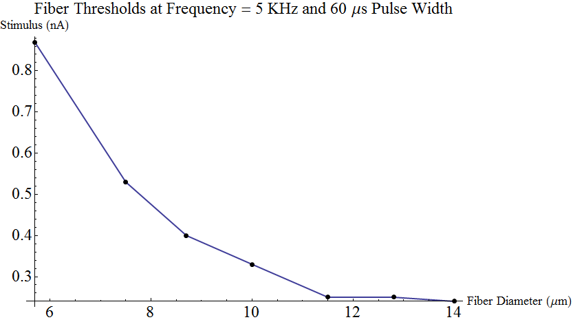
This is a plot of axon thresholds by the electrical stimulus strength on their surface that is required to fire them for various diameter axons. The stimulation is in 60 microsecond pulses, 5000 per second. Axons have little repeater stations to keep the signal going and electrical stimulation can trigger these repeaters. These are large- to medium-sized fibers that sense proprioception (muscle position) and fine-touch with a conduction velocity of 30 - 70 m/sec. The overall study is on high frequency stimulation of the spinal cord for pain relief.

ListLinePlot[
  {{5.7,.87},{7.5,.53},{8.7,.40},{10.0,.33},{11.5,.25},{12.8,.25},{14.0,.24}},
  Mesh->Full,
  MeshStyle->PointSize@Large,
  PlotStyle->Thick,
  TicksStyle->Large,
  PlotLabel->Style["Fiber Thresholds at Frequency = 5 KHz and 60 \[Mu]s Pulse Width",Large],
  AxesLabel->{Style["Fiber Diameter (\[Mu]m)",FontSize->18],   Style["Stimulus (nA)",FontSize->18]}
]

My 1985 Notes on Wolfram's Harvard Talk on SMP - Precursor to Mathematica Part 2

Continuing from pp 1 - 3. This part contains some juicy tidbits that show how the principles underlying Wolfram's vision of a mathematical computer language have guided Mathematica's development to this day.

  

SMP contains the core of mathematical knowledge. A library of external files extends knowledge and gives definitions for particular applications; currently about 400 files.

Has a simple algorithm to strip to word roots and search a keyword index.

"This is a language, not something that thinks, and it was designed to be easy to tell things to it."

Dimensional analysis for physical units; fundamental units and derived terms' units.

Euler circuit in a graph (?)

Laplacian and divergences computed in various types of coordinate systems.

Routine mathematics should become as computerized as arithmetic.

SMP will run on a new generation of PCs.

One can typically define a hierarchy of types of objects. Then coerce two types to a common ancestor on a graph of types. How to get to the common ancestor? There may not be a unique path, so need a weighting function to [add efficacy to the search].

Vectorize: adds arrays of numbers in same number of operations as adding single numbers.

When to swap data with disc is left to the operating system. SMP needs a C compiler to work.

Gamma matrix manipulation.

Non-Q Predicates in Mathematica

There are Predicates that are not given the Q suffix, which is an inconsistency in the nomenclature.

Numerical Non-Q Predicates

Less
Greater
Positive
Negative
Divisible
DiscreteDelta
KroneckerDelta

String Non-Q Predicates

NumberString
DigitCharacter
LetterCharacter
WordCharacter
WordBoundary
HexadecimalCharacter
WhitespaceCharacter
StartOfLine
EndOfLine
StartOfString
EndOfString

ApplyAll Applies a Function to all Subexpressions at Level One

ApplyAll

Instead of applying a function f to an entire expression, i.e. replacing the Head of the expression with f, use ApplyAll like Map to apply the function to each subexpression at level 1 of the expression. Apply defaults to Level 0 (the Head) and ApplyAll is just a convenient shorthand for Apply[ f, expr, 1].

Here is a typical example of ApplyAll. You have a List of number pairs and you want to perform some arithmetical operation such as add, multiply, divide, raise one to the power of the other, etc. (To remember the syntax of RandomReal I think of its arguments sequentially in English: "give me random reals between 1 and 20, 10 of them with length 2" (i.e. a 10 x 2 array).)

pairs=RandomReal[{0,1},{20,2}]

{{0.00994214,0.0701189},{0.024718,0.24013},{0.434799,0.996965},{0.323499,0.444366},{0.799502,0.843786},{0.964146,0.254526},{0.438815,0.943254},{0.228569,0.00348145},{0.247675,0.773157},{0.879202,0.615889},{0.898872,0.232664},{0.381568,0.75334},{0.464207,0.659948},{0.843115,0.179364},{0.287139,0.636774},{0.922514,0.193705},{0.969753,0.273868},{0.012059,0.247027},{0.560162,0.962637},{0.0593815,0.331142}}

Map doesn't work. It essentially disappears because it has no effect on a List:

Plus[List[a,b]]

{a,b}

Plus/@pairs

{{0.00994214,0.0701189},{0.024718,0.24013},{0.434799,0.996965},{0.323499,0.444366},{0.799502,0.843786},{0.964146,0.254526},{0.438815,0.943254},{0.228569,0.00348145},{0.247675,0.773157},{0.879202,0.615889},{0.898872,0.232664},{0.381568,0.75334},{0.464207,0.659948},{0.843115,0.179364},{0.287139,0.636774},{0.922514,0.193705},{0.969753,0.273868},{0.012059,0.247027},{0.560162,0.962637},{0.0593815,0.331142}}

But ApplyAll works perfectly; we always use its abbreviated version:

Plus@@@pairs

{0.080061,0.264848,1.43176,0.767865,1.64329,1.21867,1.38207,0.23205,1.02083,1.49509,1.13154,1.13491,1.12416,1.02248,0.923913,1.11622,1.24362,0.259086,1.5228,0.390524}

Times@@@pairs

{0.000697132,0.00593553,0.43348,0.143752,0.674608,0.2454,0.413914,0.000795751,0.191491,0.541491,0.209135,0.287451,0.306352,0.151224,0.182842,0.178696,0.265585,0.00297889,0.539232,0.0196637}

Here is a another example of ApplyAll. I want to make a toy directed graph so I can explore the new graph functions that have superseded the Combinatorica package as of Version 8.

randomEdges=RandomInteger[{1,20},{10,2}]

{{16,5},{17,17},{10,10},{15,2},{9,8},{20,9},{19,7},{20,15},{8,20},{11,3}}

Now I want to convert the pairs of numbers into a directed graph with DirectedEdge. My first try fails, again because each subexpression is a List.

toyGraph=DirectedEdge/@randomEdges

{DirectedEdge[{16,5}],DirectedEdge[{17,17}],DirectedEdge[{10,10}],DirectedEdge[{15,2}],DirectedEdge[{9,8}],DirectedEdge[{20,9}],DirectedEdge[{19,7}],DirectedEdge[{20,15}],DirectedEdge[{8,20}],DirectedEdge[{11,3}]}

What I need is ApplyAll.

toyGraph=DirectedEdge@@@randomEdges

It is equivalent to Apply[ DirectedEdge, randomEdges, 1].

Apply[DirectedEdge,randomEdges,1]

My 1985 Notes on Wolfram Harvard Talk on SMP - Precursor to Mathematica Part 1

Here is more Mathematicana to celebrate Mathematica's 25th Anniversary. Thanks to my friend and intellectual complement John Deming ('you might be interested in this'), I was present at the creation, at least to hear, with growing excitement as I sat in Aiken 101 at Harvard in 1985, one of Stephen's early talks on the Symbolic Manipulation Program, SMP, which became Mathematica. I have it on good authority that none other than Steve Jobs, marketing genius extraordinaire, came up with the name Mathematica when Stephen solicited outside suggestions.

So here are pp 1-3 of my notes transcribed and an image. I'm sure I misunderstood some of the talk, so if in doubt check the SMP Handbook, a fascinating bit of history itself. Regarding the note that SMP was "written in 120K lines of C" as of the date of the talk, in this period Stephen could write up to 1000 lines of C code in a day.

298(85)/3/11 15:30
Harvard, Aiken 101

Dr. S. Wolfram

Arithmetic, logarithms - now hardware is powerful enough to do math generally. We need a language. Needs to be general, interactive, extensible, efficient (able to do heavy duty problems), portable (able to run without change on many computers).

Intrinsic data types: numbers, arrays of numbers. But need types for higher level objects, too, algorithms for them, and symbolic manipulation of them. An intrinsic structure to deal with these.

SMP. Symbolic Manipulation Program, which I started 5 years ago. Now it's 120K lines of C code later. SMP contains the core of a fundamental mathematical language; plus programmability allowing definitions of new objects; graphics; and a [functions] library.

The basic objects are numbers; symbols such as "a", "Pi"; projections i.e. parts of objects; and lists to specify collections of objects. Assignment of symbols to "values". You specify specific values then add more general expressions or values to which the machine goes if the specific values do not apply.

Conditions: $a_ = (test) to say $a such that (test) is true.

[Handles] multigeneric functions such as the gamma function. [Piecewise functions? But I'm not sure I got this right-KWC]

$$x stands for sequence of expressions.

It's important to have well-defined rules for pattern-matching. [SMP] will pattern-match even when not asked to solve explicit mathematical functions.

:   immediate assignment
::  delayed assignment

[Uses?] the Frobenius method of series expansion of differential equations. Total differential equations. XDSol J Greif & SW [Caltech?] Oct 1981.

Euler-Mascheroni constant.

Hypergeometric functions are very difficult to evaluate. Often evaluates to yield no value. Factorization: [uses the] fastest code written (as opposed to Berlekamp's). Integration: Risch etc algorithms.

Canonical form used for simplification. Applies the chain rule to reduce and solve differential equations.

Manipulates expressions: as trees, graphically.

List Operations: APL + symbolic operations etc.

Lends itself to building up programs instinctively, because symbolic language, unlike numerical languages (C?)...

Strongly based on pattern-matching. explicit assignment of cases [i.e. piecewise functions] is more natural and better for mathematics than a series of if-then functions.

User can define input & output syntax

Code generation: Convert SMP to C or FORTRAN for numerical cases: compile & load code incorporated; and add intrinsic code to SMP.

Written in 120K lines of C, runs under UNIX, VMS, VM...

Multi-n-ary tree internal data structure
Memory management
sub-expression sharing mechanisms
compacting garbage collection
-> intermediate expressions > ~16Mb
Block transfer.

Pp 4-5 of the notes are here and contain some fascinating insights into the principles guiding Mathematica's development to this day and beyond.

What I Gave Stephen Wolfram On His 50th Birthday

To celebrate the 25th anniversary of Mathematica's release, I will post some Mathematicana. I'll explain this chart more fully later but here is a précis. Stephen developed Mathematica in part so that he'd have a powerful tool with which to explore the targets of his curiosity. (And we benefit by having a powerful tool with which to explore the targets of our curiosity!) The principal result of his explorations is A New Kind of Science (NKS for short), during the writing of which,  thanks to Mathematica, he made "more discoveries than I ever thought possible" (NKS p 22).

Until recently the history of science and separately, mathematics, displayed the great theme of logical reductionism, by which I mean our success at reducing disparate phenomena to a relatively few postulates or axioms. Viz, physics, or mathematics. While Wolfram's key discovery was that a short sequence can generate unlimited complexity (NKS Ch 2) and while "short sequence" does imply reductionism, the unlimited complexity is anti-reductionistic. To expose the phenomena described by some short sequences we must compute them interminably. This chart, an attempt to place NKS in history, is what I gave Stephen on his birthday several years ago (click to enlarge).

The "flowstream" term is from the lectures of Andrew J. Galambos, a great, but largely unsung, philosopher. When I mentioned the concept of an intellectual flowstream to my friend Dave Waltz, he pointed me to the fascinating work of Eugene Garfield, notably the Web of Science.

How It Works: First, Last, Rest, Map, Apply, Nest, Fold

I adapted these functions from exercises in David Wagner's superb book, Power Programming in Mathematica, now out of print, recommended by MathGroup.

The first four are examples of an axiom of primitive and general recursive functions, projection (see Gray, p. 411), but also of selectors, functions used in a data structure to access data in a controlled way without altering the data itself (see Maeder).

myFirst@head_[first_,last___] := first

myLast@head_[most___,last_] := last

myMost@{most___, last_} := {most}
myMost@head_[most___,last_] := {most}

myRest@head_[first_,rest___] := {rest}

Here is how Apply works:

myApply[f_, head_@anything___] := f@anything
myApply[f_, anything_] := f@anything

Recursive Definitions for Map, Nest, Fold

Note the piecewise definitions and use of recursion for Map, Nest, and Fold, which work so elegantly. Before seeing Wagner's solutions I thought these functions must use a procedural-type of iteration and list decomposition.

myMap[f_,{a_,b___}]:= Join[{f@a},myMap[f,{b}] ]
myMap[f_,{}]:={}  (* base case *)

myNest[f_,x_,n_Integer?Positive]:= myNest[f,f@x,n-1]
myNest[f_,x_,0]:= x  (* base case *)

myFold[f_,x_,{a_,b___}]:= myFold[f,f[x,a],{b}]
myFold[f_,x_,{}]:= x  (* base case *)

Recursive, Rule-Based Definitions for Map, Nest, Fold

Here are Map, Nest, and Fold using a "pure" rule-based approach, meaning using only rules and patterns. Wagner notes that it turns out that Map is the most difficult of them to implement this way.

Clear[myNest,myFold,myMap];

myNest[f_,x_,n_Integer]:= {x,n}//.{{a_,0}:>a,{a_,b_}:>{f@a,b-1}}

myFold[f_,x_,s_List]:= {x,s}//.{{a_,{}}:>a,{a_,{b_,c___}}:>{f[a,b],{c}}}

myMap[f_,s_List]:= Module[{r},{s,{}}//.{{{},r_}:>r, {{a_,b___},r_}:>{{b},Append[r,f@a]}}]

Getting Help: Find a Function Using Wildcards

There are over 4000 built-in functions in Mathematica, not including those in add-on Packages. 

In[340]:= Names["System`*"]//Length

Out[340]= 4131

Therefore it makes sense to see if there is a built-in function before we write one. Likewise, the large number of functions means that we often have a vague memory of a function we've used but can't put our finger on its name when we need it again. If I have some idea of the name of a function I've used, or want to see if there is an existing function and guess at part of its name, I use a wildcard in my current Notebook with the short form of Information (?). To find a function or survey related functions, this is faster than using the Doc Center.

Here I want to know the filepath of my current Notebook, which I cannot find in any Mathematica menu item. Maybe there's a Notebook function to tell me. I scan down the results until I see NotebookFileName, which is the one I want. I also quickly click on a half-dozen or so functions to refresh my memory of them or explore new ones and read the short info displayed below the results.

Using Information this way is always fruitful for me since I efficiently learn about functions I didn't remember or didn't know. But if it fails to flush out the function I want, I go to the Doc Center and search there.

Flat (Function Attribute of associativity; removes brackets and parentheses)

Why does this function works for more than the two arguments for which it is defined?

In[100]:= log[a_ b_]:=log@a+log@b

In[101]:= log[2 x y]

Out[101]= log[2]+log[x]+log[y]

The answer is that Times has the Attribute Flat, which is Mathematica's interesting name for the mathematical property of associativity. I.e., as we learned in school, (2 + 3) + 4 = 2 + (3 + 4). We can remove the parentheses. So the Attribute is called Flat since, after the name for the function Flatten that removes List brackets, Mathematica knows that for some functions it's valid to remove all parentheses or List brackets. What is handy is to automatically remove all brackets from a user-defined function, use SetAttributes[ function, Flat].

Thus Time's Attributes show it to be more profound than we might expect. We check function Attributes like this:

In[102]:= Attributes@Plus

Out[102]= {Flat,Listable,NumericFunction,OneIdentity,Orderless,Protected}

And we can find all built-in functions with a given attribute like this, first taking all function Names from the System context where they live, using the wildcard "*", then using a pattern in Cases:

In[103]:= Names@"System`*"//Cases[#,_?(MemberQ[Attributes@#,Orderless]&)]&

Out[103]= {ArithmeticGeometricMean,BitAnd,BitOr,BitXor,CoprimeQ,DiracDelta,DiscreteDelta,Equivalent,GCD,HeavisideTheta,KroneckerDelta,LCM,Majority,Max,Min,Multinomial,Plus,Times,UnitStep,Xnor,Xor}

Last, Trace shows how the Flat Attribute affects the operation of Times in the simple example. Mathematica knows it can split up a function applied to two arguments times each other, and, typically for the evaluator, keeps applying the rule to split up all arguments of Times until there are no lists of more than two left.

In[104]:= log[2x y]//Trace

Out[104]= {log[2 x y],log[2]+log[x y],{log[x y],log[x]+log[y]},log[2]+(log[x]+log[y]),log[2]+log[x]+log[y]}

How to Write a Program in Mathematica: Basic Programming Principles

If you look at the code of the creators of Mathematica's programming language, Stephen Wolfram (e.g. Ch. 5., Cellular Automata, of A New Kind of Science) and Roman Maeder (see his superb books), you will see simplicity and organization. They are master programmers. So if the method of Wolfram and Maeder is to keep things simple and thoughtfully organize their programs, let us follow their example. With that in mind, here are some principles to create any program, step by step.

1. Write and debug a series of one liners to execute your program. In other words, start by just doing what you want to do "by hand," one line at a time. Then when you're done and it works, assemble the series of one liners into a program.
2. If the input or output of any step is at all complicated, first solve a toy version. If your entire program is complicated, first solve a toy version of it. Then try each step on the actual problem.
3. A Functional programming principle is write functions few inputs and outputs as possible–ideally just one output. If you have only one input and one output per function, each is easy to write and debug. Sometimes you have to carry related parameters together. In the function under construction, it's still advisable to have as few parameters affect a single output as possible. 
4. To assemble the program, first create the shell, i.e. just a Module (or With or Block) with the name of the program function and those of its arguments. Then put each one-liner in the program one at a time, on a separate line, and run the program. 
5. A Print statement is the simplest form of debugging. So Return or Print the output of any command that you need to see. If you have a long set of arguments or if any are complex, start by just returning the arguments to see if you get what you expected. Leave a Print statement in the program if you need to monitor each output, or if not, delete it. If you think you might need it, comment it out (*Print@variable1."*).
6. And in general, per the 2000-year old army saying, Clean As You Go (which derives from the law of increasing entropy). Precede your function with Clear@function. Delete things you don't need. Re-organize for clarity. 
7. There is no shame in clarity. Someone else may need to read your code. And you may be that someone else. As an acquaintance of mine, Gary Drescher, once said, "The 'I' of the future is only loosely coupled to the 'I' of the present." You, 6 months from now, will not have an easy time of deciphering your own code unless you go for clarity. 

• Use long variable names (like master programmers Hoare and Trott). 
• Format a cell for text (Alt+7) above your program and comment freely. 
• Use inline comments (* comment here *) judiciously alongside lines of your code. Too many comments break up the readability.
• Use the combination of Prefix and Postfix with pure Function that I advocate (here in this blog), which simplifies your code and gives you total control over which functions to emphasize and which to subordinate. 

7. As you put each one liner in the program, be sure to include any variable names in the local variable List in the Module. If variable names are not listed Mathematica will flag them in a color (blue in my version). You can save space and simplify things by putting assignment functions in the local variable List as long as they're not dependent on a variable that came earlier in the List. If they are dependent, the assignment has to be put in the program body. Put the local variable names in the List in the order that they appear in your program.

8. Remember the fundamental data structure principles:

• Write and debug a special function, called a Selector, to extract each subset of what you need from your data. Only use Selectors to touch the data; never touch it directly with the program. When the structure of your data changes, re-write the Selector.
• Write and debug a special function, called a Constructor, to build each construct from the data. Only use Constructors to build the constructs. Leave the original data alone.
• If need be, write and debug a special function to export or format the output of your program. Only use the special function to export or format your output.
• Two other arch-typical data structure functions are constants, that always return the same thing either with no input or no matter what the input, and predicates, that take an input and return True or False.

9. Whether to define a function in your program, or outside of it and then call it in the program, is a judgment call. A simple but valid answer is if you plan on using the function outside of your program, define it outside to facilitate that usage. But an equally important reason for defining a function outside of your program is to simplify it.
10. With a medium to large program, consider just throwing out the original version if you see a better approach. At an IEEE seminar on object-oriented programming, the speaker said often you just need to start coding for a bit to get a feel for what you want to do before you can envision a better architectural solution.

Obviously I need to provide examples to illustrate all these principles and will do so.

Introduction to Strings in Mathematica

A format convention in Mathematica is to show quotation marks around strings in input cells, but not in output cells. To show them in output cells, use FullForm.

In[18]:= "I've entered a string by using quotation marks."

Out[18]= I've entered a string by using quotation marks.

In[19]:= Head@%

Out[19]= String

In[20]:= FullForm@%%

Out[20]//FullForm= "I've entered a string by using quotation marks."

In programming languages, "String" is the name for the data type of text expressions. In other words, unlike symbols in a general expression, the symbols in a String, like a, b, c, do not refer to places in memory that store a variable, like a function or value. Symbols in a String do not refer to anything, or you could say they only refer to themselves as "literals", that is, the literal characters or tokens "a", "b", "c". An "a" is just a blank token with nothing behind it; hence the terms "literal" or "token" for a String symbol.

In[21]:= a = 5534.7; a

Out[21]= 5534.7

Trying to use a String as a variable gives an error message.

In[22]:= "a" = "Lookee here."

During evaluation of In[22]:= Set::setraw: Cannot assign to raw object a. >>

Out[22]= "Lookee here."

Consequently, Strings are not evaluated in the usual way that other Expressions are. Wellin et al. in their excellent book suggest that we think of a String as being broken up by Mathematica into a sequence of its characters and then functions are applied to the sequence.

In[8]:= aSentence = "The quick brown fox jumped over the 742 lazy white dogs.";

In[11]:= aSentenceCharacters = aSentence // Characters

Out[11]= {T,h,e, ,q,u,i,c,k, ,b,r,o,w,n, ,f,o,x, ,j,u,m,p,e,d, ,o,v,e,r, ,t,h,e, ,7,4,2, ,l,a,z,y, ,w,h,i,t,e, ,d,o,g,s,.}

Functions, like MatchQ, Cases, Position, etc., that work on non-String expressions do not work on Strings but do work on their sequence of characters.

In[14]:= Position[aSentence, "e"]

Out[14]= {}

So perhaps as Wellin et al suggest, Mathematica first breaks a String into a sequence of characters and applies some of the regular built-in functions as well as some specialized String functions to the sequence.


In[25]:= MatchQ[#, "e"] & /@ aSentenceCharacters

Out[25]= {False, False, True, False, False, False, False, False, False, False, False, False, False, False, False, False, False, False, False, False, False, False, False, False, True, False, False, False, False, True, False, False, False, False, True, False, False, False, False, False, False, False, False, False, False, False, False, False, False, True, False, False, False, False, False, False}

In[24]:= StringMatchQ[aSentenceCharacters, "e"]

Out[24]= {False, False, True, False, False, False, False, False, False, False, False, False, False, False, False, False, False, False, False, False, False, False, False, False, True, False, False, False, False, True, False, False, False, False, True, False, False, False, False, False, False, False, False, False, False, False, False, False, False, True, False, False, False, False, False, False}


In[15]:= Position[aSentenceCharacters, "e"]

Out[15]= {{3}, {25}, {30}, {35}, {50}}

In[16]:= StringPosition[aSentence, "e"]

Out[16]= {{3, 3}, {25, 25}, {30, 30}, {35, 35}, {50, 50}}

The position index is repeated in StringPosition since it shows the beginning and ending positions of the matched String.

In[20]:= StringPosition[aSentence, "lazy"]

Out[20]= {{41, 44}}

When working with Strings, you do not need to enclose a String in List brackets:

In[3]:= aString = {"abcd"}

Out[3]= {abcd}

In[4]:= aString2 = "abcd"

Out[4]= abcd

In[5]:= Head@aString2

Out[5]= String

The String is delimited by invisible quotation marks. As usual FullForm and InputForm reveal the way Mathematica sees the String.

In[6]:= FullForm@aString2

Out[6]="abcd"

In[7]:= InputForm@aString2

Out[7]="abcd"

Next we will look at the variety of String functions in Mathematica.