How to Lose List Brackets in Mathematica

First, Apply, Sequence, ReplaceAll

There come times in every Mathematica user's life when the all-pervasive List brackets get in the way. Sometimes it's easy to redesign the function to accept the arguments in a List. Here are other solutions.

First

For a single element enclosed by brackets, you can use First to extract the element. In this example, since all Mathematica arithmetic functions are Listable (they will automatically Map over a List) we specify that the argument must be an Integer so the function will fail.

enclosed1={2};
Clear@function1;function1@x_Integer:=x^3;
function1@enclosed1

function1[{2}]

function1@First@enclosed1

8

Apply

First, see if you can use Apply @@ to apply a function to the contents of your List. Apply will replace the List head with your desired function and Evaluate it.

In[107]:=  Range@15
Out[107]=  {1,2,3,4,5,6,7,8,9,10,11,12,13,14,15}

In[108]:=  Plus@@%
Out[108]=  120

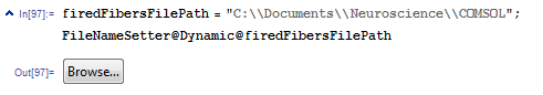
Here's a single filename that is unnecessarily surrounded by List brackets. It's a String, so we just Apply ToString to it. It then stands alone – no List brackets – but its Head is String.

FileNames[]

{TableFiredFibers-Control-CathodeOnly-0p644.txt}

ToString@@%141

TableFiredFibers-Control-CathodeOnly-0p644.txt

Head@%
String

FullForm@%%
"TableFiredFibers-Control-CathodeOnly-0p644.txt"

Sequence

Mathematica was designed as a list processing language in which the list is the fundamental data structure. Allan Newell's IPL (Information Processing Language) was the original prototype, after which John McCarthy coupled the list as a universal data structure with the lambda calculus and logic functions into the major programming language, LISP.

We can Apply Sequence to a List to replace List as the container (the Head). Here are two examples, first to a single List, then to a List of Lists.

In[115]:= Sequence@@{0,4}

Out[115]= Sequence[0,4]

In[119]:= Sequence@@{{0,1,1},{0,2},{0,1,3},{0,4}}

Out[119]= Sequence[{0,1,1},{0,2},{0,1,3},{0,4}]

FileNameJoin is the safe way to assemble filepaths in Mathematica since it knows your operating system syntax. However FileNameJoin only accepts a single-level List as its argument. To feed it a nested List, use Sequence instead of List as the Head of the inner List.

In[350]:= twoPathElements={"webPages","index.html"};

In[351]:= FileNameJoin@{$HomeDirectory,twoPathElements}

Out[351]= FileNameJoin[{C:\Users\kwcarlso,{webPages,index.html}}]

Since it didn't see a List of Strings (filepath names) as the correct argument types, FileNameJoin returned the input. Using Sequence solves this.

In[352]:= twoPathElements=Sequence["webPages","index.html"];

In[353]:= FileNameJoin@{$HomeDirectory,twoPathElements}

Out[353]= C:\Users\kwcarlso\webPages\index.html

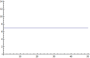
The context of one function I use to illustrate Sequence is worth mentioning (but skip this to get to more usages of Sequence). I have digitally sampled a curve from the literature (a paper by Holsheimer from 1999) in the graphing program Origin. In other words, you can import an image, in this case a graph for which Holsheimer doesn't give either the underlying data or an equation, and repeatedly click on it to harvest {x,y} values. We captured 163 sample points on the solid curve below, which is a vast improvement on the antiquated method of using a straightedge to pick up x and y values off the axes.

With that many sample points, finding the x value closest to the one desired is a reasonable alternative to fitting a curve and applying the fit equation to values you wish to interpolate or extrapolate.

So this is a function to find the nearest x value (a neuron axon diameter, fiberDiameter) to one for which we want to know the threshold as determined by Holsheimer (which is the y-value retrieved). The problem is Nearest returns values in List brackets, which don't match the un-bracketed x values in the List of data. Applying Sequence to the result of Nearest feeds the unbracketed value to Cases, which then performs the match.

Clear@diameterThreshold; diameterThreshold[fiberDiameter_, fiberThresholdSourceData_:holsheimerData1999] := Cases[fiberThresholdSourceData, {x_, y_} /; x == Sequence@@Nearest[fiberThresholdSourceData[[All, 1]], fiberDiameter] ]

So in sum this function says: Clear the function name (which I do habitually at the start of a function definition to prevent accidentally testing a previous version as I revise it). Then define it as the Cases in the source data file (fiberThresholdSourceData--default to the holsheimerData1999 file unless I specify another file) such that ( /; ) the x-value is Nearest to the fiberDiameter parameter I give it.

ReplaceAll

Here is a third way using rule patterns.

In[128]:= {{0,1,1},{0,2},{0,1,3},{0,4}}/. List[a__] ->a

Out[128]= Sequence[{0,1,1},{0,2},{0,1,3},{0,4}]

Mathematica Keyboard Shortcuts

Keyboard Shortcuts and Handy Short Commands

Here are some useful and lesser-known keyboard shortcuts. In terms of saving time, rather than using brackets for single-argument functions, use Prefix: function@argument.

Likewise, nesting functions with increasingly distal matched brackets is difficult to read, increases programming time, and obstructs you highlighting what you feel is important in the function. Use Postfix-style with pure Functions like this:

dataFiles[[1]]//Rest//Flatten//Length;

dataFilesDifferences//Chop[#,10^-4]&//Union/@#&//ListPlot/@#&//Partition[#,3]&//Grid

As advocated in my 2007 User Conference talk (also here), a "Functional-Procedural Fusion" elegantly represents deeply nested functions in a readable manner. If you do use deeply nested functions, multiple-clicking the Head of an Expression will select its brackets.

Ctrl+F6          Switch between open Mathematica notebooks
F12                Toggle current notebook to and from full screen

Ctrl+Shift+K  After a function name gives you a template for the simplest form of the function

Ctrl+K            After a function name gives a drop-down listbox with autocompletions of the function

?*name*         As in "?*Plot*" lists all Mathematica functions with Plot in their name. You can then click on them to get quick help text.

?Global`*       Lists all Names created in current Mathematica session

F1                  Search Help for expression to left of cursor

Shift + F1      Open new instance of Help browser. Do scratchpad calcs in Help rather than opening a new Notebook. They're automatically cleaned up when you go to a new Help topic.

Alt+.              Interrupt a computation. If it doesn't work, do Evaluation/Quit Kernel.
Shift+Alt+.    Remove a selected computation from the Evaluation queue. This is handy when you have a long computation running, start another one, and want to abort that one without aborting the one that is running.

Rather than using palettes, just learn keyboard shortcuts for the symbols you use frequently, for example:

esc+[character}+esc  E.g. to give the Greek letter corresponding to the keyboard character
Ctrl+6             Superscript
Ctrl+-              Subscript
Alt+7              Format cell as plain text
Alt+6              Format cell as Subsubsection
Alt+5              Format cell as Subsection

%+Out line    As: %127. Refers to output line #127. Same as Out@127 or Out[127] but more concise. I use this frequently for a temporary variable name but if it turns out I need a more permanent mnemonic name I just create one: newName = %127. I use %, %%, or %2 only for very temporary "scratchpad" calcs.

Ctrl+L            Copy input cell from the one just above
Ctrl+Shift+L   Copy output cell from the one just above, into new input cell. An alternative is to just start typing in the Output cell and Mathematica automatically creates a new Input cell with those contents.

Clear@%127  Removes from memory some huge expression you created or imported in In[127].
ClearAll["Global`*"] and Remove["Global`*"] Clears or Removes all values from variables you created in the current session. If it comes to that, I usually kill the kernel though (Evaluation/Quit Kernel).

filePath="C:\\directory1\\directory2"; FileNameSetter@Dynamic@filePath

Gives you a in-Notebook button to click to navigate and select a filename or directory to which to Set filePath. Giving filePath an initial value before evaluating FileNameSetter takes you to that value (e.g. a directory) when you click the button. Using Dynamic lets you click the button over and over to re-Set filePath.

CreateDocument@expression Opens a new Mathematica notebook with expression in it. Expression can be an imported document.

Mathematica Plot: Using Table to See Numerical Values

Plot with Table to See Numerical Values

We saw how to use Table to generate sample points for a ListPlot, and how to compare your own sample to Plot showing its mesh points. Here is the converse usage, using Plot to graph a function and then Table to see it numerically. We'll start with a simple sine curve.

To see numerical values, I click Control+L to regenerate the input, replace "Plot" with "Table", and specify a third argument for the iterator to give the sampling frequency. The Postfix function N tells Mathematica to give us decimal output instead of its default, exact fractional values.

In[314]:= Table[{x, Sin@x // N}, {x, 0, 2 Pi, Pi/4}] // TableForm

Let's look at a more complicated example with two decay curves that are identical except for their asymptotes, which are 0 for decay1 and 0.7 for decay 2 (shown in the Plot).

In[347]:= Clear@decay1; decay1@d_ := (q/d) + 0.7; q = .2;

In[348]:= Clear@decay2; decay2@d_ := (q/d); q = .2;

In[363]:= Plot[{decay1@d, decay2@d}, {d, .1, 4}, PlotRange -> {Automatic, {0, 3}}]

When you need to keep track of three or more columns, TableHeadings can be helpful. Here we say no row headings, but three column headings.

Table[{d, decay1@d, decay2@d}, {d, .1, 1.2, .1}] // 

 TableForm[#, TableHeadings -> {None, {"d", "decay1@d", "decay2@d"}}] &

Mathematica Plot: Options Overview

Plot Has over 80 Options to Control its Behavior


Here is a Plot of two curves where we use Plot options to add a Frame, tick marks to the left and right y-axes, but to the bottom x-axis only, and to Plot the full -y-range instead of leaving out extreme values.

Plot[Tooltip@{Sin@x, x Sin@x}, {x, 0, 20}, Frame -> True,
 FrameTicks -> {{Automatic, All}, {Automatic, None}}, PlotRange -> Full]

You can ask Mathematica for all the available Options for a function with Options@function. When you do, Mathematica tells you their default values as well.

Options@Plot // Partition[#, 3,3,1,{}] & // TableForm

The Partition syntax may look a little complicated, but is explained in Capturing the Remnant of a Partitioned List. It says: "Partition the list into sublists of length 3, take them in blocks of 3 (i.e. do not overlap them), start the first element of the first list at position 1 of the first sublist (at the beginning), and do not pad the last uneven list (i.e. pad it with the empty set)." While Plot has 57 Options, which divide evenly by 3, the partition syntax will work if Plot has a non-divisible-by-3 number of Options in the future.

I thank a diligent reader, Murta, for suggesting this correction to my original post.

Plotting Constant Functions

Plotting Constant Functions


You may want to plot a constant, for instance to combine with another plot. To do this you specify the constant without a function and the domain within which you want to plot the function.

Plot[5, {x, 0, 5}]

Suppose you want to plot a constant x value for all y. That's not a function and Plot won't work. For instance, you may want to plot a vertical asymptote and while Mathematica will plot vertical asymptotes for some functions (see the plot for Tan@x in tutorial/Basic Plotting), it may not for all. Here is one method. Note that any number followed by pure Function "&" makes a constant Function for that number's value. In other words, the constant Function yields the constant no matter what number it is applied to.

4.5 & /@ {5, 28.6, Pi, E}

{4.5, 4.5, 4.5, 4.5}


Here we use the constant pure Function to create the x-values as just shown. Thread with List creates the 50 pairs of y-values for x = 7.

Thread[List[7 & /@ Range[0, 50], Range[0, 50]]] // Short

{{7,0},{7,1},{7,2},{7,3},{7,4},{7,5},{7,6},{7,7},<<35>>,{7,43},{7,44},{7,45},{7,46},{7,47},{7,48},{7,49},{7,50}}

ListLinePlot[Thread[List[7 & /@ Range[0, 50], Range[0, 50]]]]

And so this is also a way to plot a constant y value by using the constant Function for the range instead of the domain.

ListLinePlot[Thread[List[Range[0, 50], 7 & /@ Range[0, 50]]]]

Mathematica Plot: Plotting More than One Function

Using Plot to Plot More than One Function


It is often useful to Plot different function parameter values and compare them. Just give Plot a list of functions with the parameter values you wish to compare and it will Plot them together without your having to use Show. Let us use the function defined in Basic Plotting:


f[x_, t_] := x^t;


You can use Table to automate the parameter sweep, but pre-generate the sweep functions or (for reasons I don't understand) Plot won't automatically color-code them.

In[278]:= sweepFunctionTable = Table[f[x, t], {x, 2, 5}]

Out[278]= {2^t, 3^t, 4^t, 5^t}

In[279]:= Plot[sweepFunctionTable, {t, 0, 5}]

Plot with Tooltip to Identify the Plots

Sometimes you can lose track of which function is which when plotting several function together. Plot helps by color-coding them. But adding Tooltip labels is another technique. Let's compare the three functions Sin x, Cos x, and Sin x + Cos x. You will need to Plot this yourself in a Notebook to mouseover and see the tooltips that label each curve with the three function names ("Sin@x", "Cos@x", "Cos@x + Sin@x").

Plot[Tooltip@{Sin@x, Cos@x, Cos@x + Sin@x}, {x, -3 Pi, 3 Pi}]

Now let's specify that the tick marks should be labeled in radians:

Plot[Tooltip@{Sin@x, Cos@x, Cos@x + Sin@x}, {x, -3 Pi, 3 Pi},
 Ticks -> {{-3 Pi, -2 Pi, -Pi, 0, Pi, 2 Pi, 3 Pi}, Automatic}]

Mathematica Plot - Basic Plotting

Plot

For starters, be aware that Mathematica's data plotting functionality is extensive and there are a variety of Plot functions. Using Information "?" with the wildcard characters "*" shows all functions that include "Plot". I won't show them here, but you can execute the command if you wish to see them.

?*Plot*

Basic Plotting

Let's say you have a function and you want to understand its behavior. We'll do a simple one.

In[238]:= y == x^n // TraditionalForm

Out[238]//TraditionalForm= y==x^n

Let's start by generating a few sample points of the function and plotting them.  You might think in the age of computers we can dispense with plotting sample points and just let Plot do the job. But when Plot fails to give you output and you don't know why, one measure is to go ahead and plot a few sample points by hand and compare them to what Plot is doing. So let's generate the sample points the easy way with Table. We Clear the function name, define the function, give x a value of 2, and use Table to sample the domain from -5 to 5 in increments of 0.5.

In[249]:= Clear@f; f[x_, t_] := x^t;

In[250]:= samplePoints = Table[f[2, t], {t, -5, 5, .5}]

Out[250]= {0.03125, 0.0441942, 0.0625, 0.0883883, 0.125, 0.176777, 0.25, 0.353553, 0.5, \
0.707107, 1., 1.41421, 2., 2.82843, 4., 5.65685, 8., 11.3137, 16., 22.6274, \
32.}

Now we plot these values using ListPlot. Ignore for now the x-tick points, which are just the number of the data point in the List.

In[242]:= plot1 = ListPlot@samplePoints

To better visualize the function, it's often helpful to connect the sample points. We use ListLinePlot. Another way is to use ListPlot's option, Joined -> True). If you look closely, you can see that the sample points are joined by line segments; our plot is not a continuous curve. Again, ignore the abscissa values.

plot2 = ListLinePlot@samplePoints

If we wished, we could combine the plots with Show--one of the most commonly-used plot techniques.

Show[plot1, plot2]

And this is similar to what Plot does--sampling a function and plotting the connected sample points--but of course in a much more sophisticated way. For one thing, Plot samples more frequently where it thinks it might need to, such as where the value of the function changes more frequently, maybe with several tries, and automatically connects the sample points in a continuous curve. Using Plot the x-axis values are correctly labeled.

Plot[f[2, t], {t, -5, 5}]

But notice that Plot is not showing the full domain and range that we asked for. By default it tries to, in effect, show the most important part of a function by excluding what it thinks might be outliers. Two options allow you to override this behavior. PlotRange->Full tells Plot to not clip the y-axis. PlotRange->All tells Plot to include all domain points and their y-values. I usually use PlotRange->All.

Plot[f[2, t], {t, -5, 5}, PlotRange -> All]

If you wish, reveal the sample points with the Option, Mesh->All. When you don't understand what Plot is doing, revealing the Mesh is a good first step. And then as I said above, you can compare Plot's sample points to yours, which might illuminate what's going on. There are more Mesh options to allow you to control how Plot uses its sample points.

Plot[f[2, t], {t, -5, 5}, Mesh -> All, PlotRange -> All]

Next: Using Plot to Plot More than One Function

Getting Help: Mathematica User Groups

MathGroup

MathGroup, www.mathgroup.org, is the original Mathematica usegroup founded and moderated by Stephen Christensen. This high-quality bulletin board is a treasure trove of invaluable Mathematica know-how, and an incredibly useful resource for answering your Mathematica questions and problems. Introduction and instructions for subscribing and posting can be found from here: http://forums.wolfram.com/mathgroup/.

StackExchange Mathematica

There is a newer Mathematica usegroup in the StackExchange group of collaboratively edited question and answer sites: http://mathematica.stackexchange.com/. Their intro says : "Welcome! This is a collaboratively edited question and answer site for users of Mathematica. It's 100% free, no registration required." The functionality of the StackExchange sites is interesting (http://stackexchange.com/sites).

File Operations: Deleting Files

Delete one or more files

DeleteFile deletes one file, or more files if they are given in a List. If you are deleting more than one file, typically you'd first use FileNames to acquire those files from a directory. DeleteFile returns Null (i.e. nothing) if it works and $Failed if it doesn't. To delete a few files in the current directory it's as simple as this.

FileNames["test*", "C:\\Users\\82V\\Documents"] // DeleteFile

Here is a more complicated example in which I delete 3500 files in multiple directories.


Acquire FileNames and Delete Files in all subdirectories

The usual sequence of steps goes like this. Set the directory in which you want to search for files. In Windows, I usually use Windows Explorer to navigate to the directory, then click in the address bar to select it, Ctrl+C to copy it, and paste it after a quote mark in Mathematica, which says to me:

In[114]:= SetDirectory@
  "C:\\Users\\82V\\Documents\\Neuroscience\\Arle-Shils\\commandUNCuS\\\
DataFiles";

Search for all the files using a wildcard and store their names in a variable (datFiles). Search in all subdirectories within your directory by using a wildcard for subdirectory names in the optional second argument, and Infinity for depth of subdirectories in the optional third argument.

In[97]:= datFiles = FileNames["*.dat", {"*"}, Infinity];

See how many filenames you captured.

In[98]:= datFiles // Length

Out[98]= 3594

Take a quick peek at the first five files to be deleted to make sure you're capturing the right ones.

In[99]:= datFiles[[1 ;; 5]]

Out[99]= {"Short_Test_File\\tc125_101.dat", "Short_Test_File\\tc125_101pre.dat", \
"Short_Test_File\\tc125_102.dat", "Short_Test_File\\tc125_102pre.dat", \
"Short_Test_File\\tc125_103.dat"}

Delete all the files to be deleted.

In[100]:= DeleteFile@datFiles

Reset the directory to whatever it was before you set it to the one in which to search for files.

In[112]:= Directory[]

Out[112]= "C:\\Users\\82V\\Documents\\Neuroscience\\Arle-Shils\\commandUNCuS\\DataFiles"

In[113]:= ResetDirectory[]

Out[113]= "C:\\Users\\82V\\Documents"

Note that if you set the directory n times to delete files in each, you need to repeat ResetDirectory[] that many times to get it back to where it was, since each time you set a directory it pushes the previous ones down a stack (which you can reveal using DirectoryStack[]), and each time you use ResetDirectory[] it pops the directories back up the stack. You can use a Do loop on ResetDirectory[] n times to do this. Using the Print statement will show you the pop sequence of directories you have visited. I prefaced the command with Directory[] to show the current directory first.

In[117]:= Directory[]; Do[Print@ResetDirectory[], {3}]

C:\Users\82V\Documents\commandUNCuS

C:\Users\82V\Documents\Neuroscience\Arle-Shils\commandUNCuS\DataFiles

C:\Users\82V\Documents

A Mathematica Bibliography, Part 1: How to Use Mathematica and its Programming Language

(Update here without annotations)

Consider reading Steve McConnell's book, cited under Programming and Computer Science books, in parallel with these if you undertake any serious programming task or just for the enjoyment and edification of learning programming best practices. I am reminded of the beautiful remark I heard by Marvin Minsky in one of his AI classes: "Anyone who doesn't program is missing one of the more interesting cultural experiences of our time."

Abell, Martha L., Braselton, James P., and Rafter, John A., Statistics with Mathematica (San Diego: Academic Press, 1999). Good introduction even though now dated due to the huge inclusion of statistics functions in Mathematica 8.

Blachman, Nancy R., and Williams, Colin P., Mathematica, A Practical Approach (Upper Saddle River NJ; Prentice Hall PTR, 1999). Introduction for beginners. I started with this book.

Dick, Samuel, Riddle, Alfred, and Stein, Douglas, Mathematica in the Laboratory (Cambridge: Cambridge University Press, 1997). An overview of using Mathematica with laboratory data and instruments. But also has excellent practical guidance on importing and exporting files and data, and file operations, and a good introduction to fitting data although you should look at the new tutorials, such as tutorial/CurveFitting for the basics, and tutorial/StatisticalModelAnalysis for more advanced analysis.

Gray, John W., Mastering Mathematica, Programming Methods and Applications 2nd edition (San Diego: Academic Press, 1998). For beginners to experts.

Maeder, Roman E., Programming in Mathematica 3rd edition (Reading MA: Addison-Wesley, 1997). Maeder was the key player in designing the Mathematica programming language with Wolfram, which I consider a major scientific and linguistic synthesis. He then showed how to use the language in significant programming areas and wrote the Wolfram Education Group course on Programming in Mathematica. I have to say, leaving a comparison of importance to history, that this is like Halley or Newton's other followers showing how to use his synthesis, e.g. to calculate the orbit and time of return of a comet. Maeder's approach is elegantly concise, high-level, and to the point.

Mangano, Sal, Mathematica Cookbook (Sebastopol, CA, USA: O'Reilly, 2010). This is my current favorite book to sample for edification and pure enjoyment. I'd say most of it is for intermediate to advanced users.

Trott, Michael, The Mathematica GuideBook for Programming (New York: Springer, 2004).  For beginners to advanced users. I've read most of this book and Trott's style, like Wolfram's, has had a strong influence on my programming style. In particular, I follow Hoare and Trott toward the goal of writing code that can be read like prose, such as using long, descriptive variable names instead of abbreviations. This is one of four 1000-page tomes by the truly prolific Trott, who also compiled the astonishing 310,000-function Wolfram Functions site http://functions.wolfram.com. Until I saw a single individual walking down the hall at the 2007 WRI Technology Conference with a badge saying "Michael Trott," I really didn't think he could be one person. I thought he must be another Bourbaki, the legendary French mathematical collaborative that published under that name.

Wagner, David B., Power Programming with  Mathematica: The Kernel (New York: McGraw-Hill, 1996). Truly a classic to which I was introduced by MathGroup.

Wellin, Paul, Gaylord, Richard, and Kamin, Samuel, An Introduction to Programming with Mathematica (Cambridge: Cambridge University Press, 2005). For beginners to intermediate users. As clear as can be. Paul Wellin heads the Wolfram Education Group.

Wolfram, Stephen, A New Kind of Science (Champaign, IL: Wolfram Media, 2002). I include NKS (as it's known), even though it's an advanced tome, because the code that is downloadable from the book's website is as exemplary for good functional programming as can be found anywhere. For instance, the simple, elegant development of the code that led to what is now CellularAutomaton and TuringMachine at the start of Chapter 5 had a major influence toward simplifying my programming style and approach to programming as a series of "one liners" (q.v. http://blog.wolfram.com/2011/12/01/the-2011-mathematica-one-liner-competition/ by my WRI namesake, Chris Carlson).

How It Works: DeleteDuplicates

Delete Duplicates

While Union is commonly used to select all unique elements from a List, including a set of Lists, DeleteDuplicates is commonly used to select unique elements from a single List, which Union can do, too. Union sorts the result, while DeleteDuplicates leaves the result in its original order. Consequently, DeleteDuplicates is a faster function if you do not need the Sort. Both functions include an optional second argument to specify the function used to remove duplicates, which greatly increases their power and versatility. First, here is DeleteDuplicates' basic functionality.

DeleteDuplicates@{c,a,b,d,a,c,a,e,e,a,a,e}

{c,a,b,d,e}

Note that if you do feed DeleteDuplicates a set of Lists, you do need to enclose the Lists in curly brackets.

DeleteDuplicates[{c,a,b},{d,a,c},{a,e},{e,a},{a,e}]

DeleteDuplicates::argb: DeleteDuplicates called with 5 arguments; between 1 and 3 arguments are expected. >>

DeleteDuplicates[{{c,a,b},{d,a,c},{a,e},{e,a},{a,e}}]

{{c,a,b},{d,a,c},{a,e},{e,a}}


You can use DeleteDuplicates' second argument to increase its breadth by specifying how it will detect the duplicates. So in the example above, by default neither Union nor DeleteDuplicates treats Lists with the same elements as equivalent, as would be the case in set theory, while this can be done with their sameness test.

It is relatively straightforward to construct the second argument if you keep in mind that the default is DeleteDuplicates[expr, SameQ] and therefore extensions of the function can take the form DeleteDuplicates[expr, f@#~SameQ~f#2&], where the comparison function f can be as complex as you wish. Here we need Sort because:

{a,b}~SameQ~{b,a}

False

DeleteDuplicates[{{c,a,b},{d,a,c},{a,e},{e,a},{a,e}},Sort@#~SameQ~Sort@#2&]

{{c,a,b},{d,a,c},{a,e}}

Here is a second, neat example from the Doc Center. Extending the power of DeleteDuplicates, this function uses Equal instead of SameQ, possibly since Equal will yield True for Reals and non-Reals. I've modified the example to show that.

5==5.

True

5===5.

False

list1 = {{0,0,0,1,0},{1,0,1,0,1},{1.,1.,1.,0.,0.},{0,0,0,0,1},{1,1,1,0,1}};

DeleteDuplicates[list1,Total@#==Total@#2&]

{{0,0,0,1,0},{1,0,1,0,1},{1,1,1,0,1}}

Here is a potential issue that limits the power of DeleteDuplicates. Trace tells us that the second 4 gets removed before it can be compared to the 16.

squaresList=Table[{x,x^2},{x,2,4}]//Flatten

{2,4,3,9,4,16}

DeleteDuplicates[squaresList,#2==#^2&]//Trace
{{squaresList,{2,4,3,9,4,16}},DeleteDuplicates[{2,4,3,9,4,16},#2==#1^2&],{(#2==#1^2&)[2,4],4==2^2,{2^2,4},4==4,True},{(#2==#1^2&)[2,3],3==2^2,{2^2,4},3==4,False},{(#2==#1^2&)[2,9],9==2^2,{2^2,4},9==4,False},{(#2==#1^2&)[2,4],4==2^2,{2^2,4},4==4,True},{(#2==#1^2&)[2,16],16==2^2,{2^2,4},16==4,False},{(#2==#1^2&)[3,9],9==3^2,{3^2,9},9==9,True},{(#2==#1^2&)[3,4],4==3^2,{3^2,9},4==9,False},{(#2==#1^2&)[3,16],16==3^2,{3^2,9},16==9,False},{2,3,16}}

We're asking DeleteDuplicates to do something beyond deleting duplicates. We should use DeleteCases to do this job.

DeleteCases[squaresList,x_/;(Sqrt@x//IntegerQ)]

{2,3}

How It Works

Somewhere Roman Maeder gives a solution to deleting duplicates and implies that his solution is efficient. From memory here is the solution (with my more efficient syntax). We create a simple list of duplicate integers.

dupeList = Table[{i, i}, {i, 10}] // Flatten

{1, 1, 2, 2, 3, 3, 4, 4, 5, 5, 6, 6, 7, 7, 8, 8, 9, 9, 10, 10}

We partition them into sets of two with offset 1 (meaning overlap of one on the original List).

dupeListPartitioned2Offset1 = Partition[dupeList, 2, 1]

{{1, 1}, {1, 2}, {2, 2}, {2, 3}, {3, 3}, {3, 4}, {4, 4}, {4, 5}, {5, 5}, {5, 6}, {6, 6}, {6, 7}, {7, 7}, {7, 8}, {8, 8}, {8, 9}, {9, 9}, {9, 10}, {10, 10}}

Now it's a simple matter to Select the sets where Part 1 is not the same as Part 2. Select always takes a predicate, sometimes of the form testQ, but here with an abbreviated operator, UnsameQ. Unequal would work for numerical entries, but UnsameQ will also work for symbols and Strings.

dupeListdupeSetsDeleted = Select[dupeListPartitioned2Offset1, #[[1]] =!= #[[2]] &]

{{1, 2}, {2, 3}, {3, 4}, {4, 5}, {5, 6}, {6, 7}, {7, 8}, {8, 9}, {9, 10}}

We're still left with duplicates. So we take the First entry of each set, and Append the Last entry of the Last set, which would have been left out. I remember thinking at this point that I would have spent time trying to not 'hack' this last part--somehow capture that last entry without another operation--but if it's good enough for Maeder, it's good enough for me. The lesson is to do what is expedient and move on to the next task.

Append[First /@ dupeListdupeSetsDeleted, Last@Last@dupeListdupeSetsDeleted]

{1, 2, 3, 4, 5, 6, 7, 8, 9, 10}

DeleteDuplicates

Import Data, Parse It, and Crunch It

These days I do a lot of data import and massage it one way or another. We are unraveling an interesting technical issue: How does mild electrical stimulation of the spinal cord (aka neuromodulation) stop chronic, debilitating pain signals? No one knows. We are close to presenting the most detailed theory yet elucidated. The project was conceived by Dr. Jeffrey Arle (neurosurgeon) and Dr. Jay Shils (electrical engineer and neurophysiologist), pioneers of neuromodulation. Jeff Arle came up with the key insight into how neuromodulation might work, and it appears in concept he is right (look for our article later this year).

Researchers around the world are exploring neuromodulation for diverse disorders such as chronic pain, movement disorders, depression and drug dependence.

Drs. Arle and Shils lead the way with their new book, Essential Neuromodulation (Academic Press 2011, 504 pp), which compiles critical work by the field's major contributors and provides a springboard for the new applications.

Nick Iftimia did the initial, very detailed research on the spinal cord. I built the initial 2200-connection model and then Nick built the more sophisticated 11,000-connection model. Then I used SolidWorks computer-aided design (CAD) software to build an accurate 3D model of three spinal cord segments and various electrical stimulators, of which the "business end" is an array of platinum-iridium electrodes.

Jay Shils selected COMSOL for our finite-element analysis and I imported the SolidWorks model into it and modeled the physics, that is, the electric potential field generated by the stimulator electrode array. Then I export part of the model, import it into Mathematica, and crunch the data for further processing by Longzhi Mei, our chief programmer, who works in C++ and Java.

All that is a prelude to how I use Mathematica in just this one portion of the project (I use it extensively elsewhere, too). Here is typically how I proceed. First I set a file path.

COMSOLFilePath="C:\\Users\\82V\\Documents\\Neuroscience\\Arle-Shils\\COMSOL\\Dura Thickening-Scar Studies\\Multi-Level-Scar-Studies\\5-Level Scar Model with Revised Geometry\\Calibration to Lee";

And then a file directory path.

SetDirectory@FileNameDrop[COMSOLFilePath,-1]

C:\Users\82V\Documents\Neuroscience\Arle-Shils\COMSOL\Dura Thickening-Scar Studies\Multi-Level-Scar-Studies\5-Level Scar Model with Revised Geometry\Calibration to Lee

I might check the FileNames in the directory.

FileNames@"*.txt"

{New-Control-WhiteMatter-1p5V-300x20x300.txt,New-Control-WhiteMatter-1p65V-300x20x300.txt,New-Control-WhiteMatter-1p6V-300x20x300.txt,New-Control-WhiteMatterV-Cathode-3v_Anodes3v_300x20x300.txt,Old-Control-WhiteMatterV-300x20x300.txt,Old-Control-WhiteMatterV-30x20x30.txt}

Then, for in-Notebook use, I just use FileNameSetter to create a convenient button for navigating and selecting a file, with the familiar Windows dialog box, to process.

FileNameSetter@Dynamic@COMSOLFilePath

FileNameSetter with Dynamic allows using the button repeatedly to select different files.Therefore I might need to just check which filepath is currently assigned to the variable, COMSOLFilePath.

COMSOLFilePath

C:\Users\82V\Documents\Neuroscience\Arle-Shils\COMSOL\Dura Thickening-Scar Studies\Multi-Level-Scar-Studies\5-Level Scar Model with Revised Geometry\Calibration to Lee\VMax@-0p65.txt

Now, obviously all those housekeeping functions are preliminary to doing something interesting with the data in the file. I Import it, and, briefly, I've learned that the "Table" format usually gives me the cleanest Mathematica representation, but note that a great feature of Mathematica is that it has well over a hundred Import and Export formats.

mesh1p12=Import[COMSOLFilePath,"Table"];

I take a quick look at the data file header and first few lines of data, which in this case are {x, y, z, V} where V is electrical potential in volts.

mesh1p12[[1;;15]]

{{%,Model:,5-level-Scar-Model-revised-Geometry-Control-Finer.mph},{%,Version:,COMSOL,4.2.0.150},{%,Date:,May,28,2012,,15:57},{%,Dimension:,3},{%,Nodes:,274151},{%,Expressions:,1},{%,Description:,Electric,potential},{%,x,y,z,V,(V)},{16.3066,4.64461,-1.77884,0.001474},{16.5566,4.47377,-1.76414,0.001851},{16.3066,4.36936,-1.74021,0.00151},{16.3066,4.48662,-1.96791,0.001486},{16.8066,4.36807,-1.73984,0.002314},{16.5556,4.17127,-1.65972,0.001872},{16.6095,4.24711,-1.89929,0.001917}}

I might check the Length of the file; here the Length measures the number of finite element mesh elements plus the header lines (8 of them).

mesh1p12//Length

274159

Now I tell Mathematica to skip the header (start at Part # 9, go to the end) and then find the Minimum of just column 4, the electrical potential. 

Min@mesh1p12[[9;;,4]]

-1.12

Those are just typical Mathematica "one-liners." Now I need to do something more sophisticated, and repeatedly. The resulting function is still concise, thanks to Mathematica incorporating a high-level programming language. Just to give you an idea of what is going on, here is a slice plot of the data at one y-value. This is what the computer in your spinal cord looks like. The gray matter, which are the neurons or processors, is the internal symmetric silhouette with the "horns," and the white matter, which are the wiring or bus lines, is the ellipse surrounding the gray matter. The white matter, that is the wires, receives signals from the peripheral nerves and the brain, feeds them to the gray matter, which is the computer that processes them, and then relays them back to brain or muscle servomotors.

ListPlot[slicePlotXZ,PlotRange->All,AspectRatio->Automatic]

Here's a overview of what the function does, as it's written in my Notebook. "NaN" is COMSOL-speak for "not a number," i.e. no numerical value. Hence I want to first get rid of all those records. Then, since we are only interested in the dorsal (back) side of the spinal cord, I lose all records with x<10, leaving the back side records to Export:

"This will 1) remove all NaN entries and 2) all records in the ventral side of the cord, as determined by the reductionCriterion, which has to be in the form, for example, {x_, ___} /; x<10 . Remember the reduction criterion is taken by DeleteCase, not Cases!"

And here's the function. For my convenience and edification, I ask it to Print various things I want to watch, such as how long it takes to Import these large files, the Length of the initial file, the Length of the reduced file, how long it takes to Export the much smaller crunched file, and the size of the reduced file in bytes.

COMSOL File Reducer

Clear@COMSOLFileReducer2;

COMSOLFileReducer2[COMSOLFilePath_String,reductionCriterion_]:=

Module[{COMSOLOutputFile=COMSOLFilePath,COMSOLwhiteMatterDataFile,COMSOLwhiteMatterDataFileNoNaN,COMSOLwhiteMatterDataFileReducedDomain,exportReducedFileName},

SetDirectory@FileNameDrop[COMSOLFilePath,-1];

Print@Timing[COMSOLwhiteMatterDataFile=Import[COMSOLOutputFile,"Table"];];

Print@Length@COMSOLwhiteMatterDataFile;

COMSOLwhiteMatterDataFileNoNaN=DeleteCases[COMSOLwhiteMatterDataFile,{___,"NaN"}];

COMSOLwhiteMatterDataFileReducedDomain=DeleteCases[COMSOLwhiteMatterDataFileNoNaN, reductionCriterion];

Print@Length@COMSOLwhiteMatterDataFileReducedDomain;

Print@COMSOLwhiteMatterDataFileReducedDomain[[1;;12]];

exportReducedFileName="Reduced"<>FileNameTake@COMSOLOutputFile;

Print@Timing[Export[exportReducedFileName,COMSOLwhiteMatterDataFileReducedDomain,"Table"];];

FileByteCount@exportReducedFileName]

And finally, here is the function in operation, starting with the command line, followed by the Print statement output, which as mentioned is just for my purview. The essential functions reduces the data file to essentials and Exports it in the appropriate format. You can see how much quicker it takes to Export the crunched file of just 1.5MB compared to the Imported file, which typically is 90MB.

In[25]:= COMSOLFileReducer2[COMSOLFilePath,{x_,y_,z_,V_}/;x<10]

During evaluation of In[25]:= {113.881,Null}

During evaluation of In[25]:= 1800008

During evaluation of In[25]:= 36942

During evaluation of In[25]:= {{%,Model:,5-level-Scar-Model-revised-Geometry-Control-Finer.mph},{%,Version:,COMSOL,4.2.0.150},{%,Date:,May,28,2012,,12:29},{%,Dimension:,3},{%,Nodes:,1800000},{%,Expressions:,1},{%,Description:,Electric,potential,in,White,Matter},{%,x,y,z,V,(V)},{10.0067,-55.9804,-6.09667,0.0000541505},{10.1067,-55.9804,-6.09667,0.0000542645},{10.2067,-55.9804,-6.09667,0.0000543788},{10.3067,-55.9804,-6.09667,0.0000544941}}

During evaluation of In[25]:= {3.62,Null}

Out[25]= 1559151

Examples of Postfix Usage and Precedence Analysis

As stated in the Mathematica archives and this blog (two parts), one of the unique aspects of my book is extensive, pervasive usage of Prefix to simplify code and save keystrokes. Like any usage of abbreviated operators, this can require knowledge of operator Precedence.


First, here's a common example of abbreviated operator precedence without Prefix. Do we need parens around the exponential coefficients?

Plot[E^-r t/.{r->.5},{t,-2,10}]

The graph shows something is wrong and Precedence analysis tells us yes, we need parens.

Precedence/@{Power,Minus,Times,ReplaceAll}

{590.,480.,400.,110.}

Plot[E^(-r t)/.{r->.5},{t,-2,10}]

Here's a typical example using Prefix. Will this function work as intended? (It's from S11: What's New in Mathematica 8 by Paul Wellin.)

f1@x_ := 1/x Cos[Log@x/x]; Plot[f1@x, {x, 0, .01}]

What would speed up Precedence analysis would be seeing an operator's Precedence popup on Mouseover, like a Tooltip. And a more minor recommendation to WRI is to make Precedence Listable to avoid needing Map. But that only saves one keystroke and I'm after much bigger game by recommending extensive usage of Prefix.

A tip is to list the operators in the order they appear in your function. Then it's easier to see which are 'stickier' than if they are out of order. Anyway, using Precedence, we see that the function will work as intended.


Unprotect@Precedence; SetAttributes[Precedence,Listable]; Protect@Precedence; Precedence@{Divide,Times,Prefix}

{470.,400.,640.}


f1@x_ := 1/x Cos[Log@x/x]; Plot[f1@x, {x, 0, .01}]

Now that we know the Precedence of Prefix and Divide, we can write the following interesting usage of Range with impunity; we don't need Table or Map. It works because Divide is Listable.

Range@5/6

{1/6,1/3,1/2,2/3,5/6}

Cyclically Selecting Parts Using Mod with Offset = 1

The Doc Center notes this usage of the offset feature in Mod to cyclically select Parts. Setting offset to 1 means Part will cycle from Part #1 through the value of n instead of the expression itself (i.e. Part #0) tbrough n - 1. However I have not seen a useful application of this idiom.

In[1]:= {a, b, c}[[Mod[Range[10], 3, 1]]]


Out[1]= {a, b, c, a, b, c, a, b, c, a}

Mod

The usage of Mod is straightforward, but by "offset" the Doc Center means shifting the cycle of remainders over by the offset along the number line. Normally Mod[m,n] is equivalent to the typical infix mathematical notation m mod n, i.e. it gives the remainder of m/x  (where x is a positive integer) as cycling from 0 through n-1. Offset rotates the cycle on the number line by its value. Here is the usage with default offset of 0:

In[149]:= Mod[Range@7, 3]


Out[149]= {1, 2, 0, 1, 2, 0, 1}

Now using an offset of 1, instead of cycling through {0,1,2}, the remainder cycles through {1,2,3}:

In[151]:= Mod[Range@7, 3, 1]


Out[151]= {1, 2, 3, 1, 2, 3, 1}

Using an offset of 2, instead of cycling between 0 and 2, the remainder cycles through {2,3,4}:

In[152]:= Mod[Range@7, 3, 2]


Out[152]= {4, 2, 3, 4, 2, 3, 4}

So what should happen if we use an offset of -1? The remainder should cycle through {-1,0,1}.

In[153]:= Mod[Range@7, 3, -1]


Out[153]= {1, -1, 0, 1, -1, 0, 1}

Capturing the Remnant of a Partitioned List

When partitioning, you usually don't want to just lose the leftover part at the end of the partitions. Mathematica provides ways to overlap Lists and pad them, but often you just want to capture the remnant leftover elements at the end. Here are two ways to do that. First, we define a function to capture the remnant and then Append it to the partitioned list, for instance in a TableForm usage.

In[77]:= TableForm@Partition[Range@11, 3]
Out[77]//TableForm=

We lost 10 and 11. Let's get them back.

In[78]:= listOfNumbers = Range@11;


remnant[listOfNumbers, 3]


Out[79]= {10, 11}


In[74]:= remnant[aList_List, partitionLength_Integer] :=
 Take[aList, -Mod[Length@aList, partitionLength]]

The most compact way to write a function that requires another short function, such as remnant, is to just protect the variable name and define the function at the same time within Module's local scope list.

In[80]:= unevenListTable[aList_List, partitionLength_Integer] :=
 Module[{remnant = Take[aList, -Mod[Length@aList, partitionLength]]},
  Partition[aList, partitionLength] // Append[#, remnant] & // TableForm]


In[81]:= unevenListTable[Range@11, 3]


Out[81]//TableForm=

There is also a way using a particular Partition syntax. What this says is, "Partition the list into sublists of length 4, take them in blocks of 4 (i.e. do not overlap them), start the first element of the first list at position 1 of the first sublist, and do not pad the last uneven list (i.e. pad it with the empty set)."

In[83]:= Partition[listOfNumbers, 3, 3, 1, {}] // TableForm


Out[83]//TableForm=

To get a glimpse of how this syntax works, by way of contrast, note what happens when we tell Partition to start the first element at position 3 of the first sublist. Since the sublists are only length 3, the first element takes that third slot and then Partition creates sublists of length 3 until it runs into too few elements to do that—the remnant, which is 11—and ignores them.

In[84]:= Partition[Range@11, 3, 3, 3, {}]


Out[84]= {{1}, {2, 3, 4}, {5, 6, 7}, {8, 9, 10}}

RecurrenceTable - Introduction

RecurrenceTable defines a sequence by setting f[n+1] equal to some function of f[n], and an initial condition for f[1]. Recurrence relations are also called difference equations and the method of finite differences uses recurrence relations. These are discrete versions of differential calculus. See the excellent articles in Wolfram Mathworld.

In our computer simulations of neural circuits, while the equations governing the neurons' behavior are phrased as differential equations, in reality we compute them as difference equations. For one thing we add noise to them, and for another, in practice they contain singularities. The "forward Euler method" et cetera won't work. I suspect that many prima facie differential equations are, in practice, unsolvable, and mask an underlying reality actually described by difference equations.

Here is a comparison between Table and RecurrenceTable that simply shows how to use the syntax of RecurrenceTable.

RecurrenceTable

In[21]:= powersOfOneHalf = Table[2^-i, {i, 1, 25}] // N

Out[21]= {0.5, 0.25, 0.125, 0.0625, 0.03125, 0.015625, 0.0078125, 0.00390625, \
0.00195313, 0.000976563, 0.000488281, 0.000244141, 0.00012207, 0.0000610352, \
0.0000305176, 0.0000152588, 7.62939*10^-6, 3.8147*10^-6, 1.90735*10^-6,
 9.53674*10^-7, 4.76837*10^-7, 2.38419*10^-7, 1.19209*10^-7, 5.96046*10^-8,
 2.98023*10^-8}

In[23]:= RecurrenceTable[{a[n + 1] == .5 a@n, a@1 == 0.5}, a, {n, 25}]

Out[23]= {0.5, 0.25, 0.125, 0.0625, 0.03125, 0.015625, 0.0078125, 0.00390625, \
0.00195313, 0.000976563, 0.000488281, 0.000244141, 0.00012207, 0.0000610352, \
0.0000305176, 0.0000152588, 7.62939*10^-6, 3.8147*10^-6, 1.90735*10^-6,
 9.53674*10^-7, 4.76837*10^-7, 2.38419*10^-7, 1.19209*10^-7, 5.96046*10^-8,
 2.98023*10^-8}

We can define f[n] in terms of more than one preceding term. If so, we need to supply the initial conditions for as many terms as specify the recurrence relations. Here is a Fibonacci-type series, a different flavor defined using three preceding terms rather than two. The initial conditions can also be thought of as boundary conditions.

In[4]:= RecurrenceTable[{a[n] == a[n - 1] + a[n - 2] + a[n - 3], a[1] == 1, a[2] == 1,
   a@3 == 1}, a,
   {n, 10}]

Out[4]= {1, 1, 1, 3, 5, 9, 17, 31, 57, 105}

Beginners: Mathematica Front End, Kernel, and Notebooks

Front End and Kernel

There are two components to Mathematica: the Front End and the Kernel. Unless you decide to use a command-line (aka "text-based") interface at a terminal, you are using the graphical user interface (GUI) of Mathematica called the Front End. If you program in Mathematica, the Front End is also your programming environment. You will find the Front End to be a superior GUI and programming environment once you get used to it. However the part of Mathematica that does the computation you request through the Front End is called the Kernel. The Kernel can run on the same computer as the Front End or on remote computers.

Mathematica Notebooks 



Most often you work in a Mathematica Notebook (the filename ends in .nb). Think of a Notebook as an electronic laboratory notebook attached to a very powerful computer (the kernel). You can do almost anything you can think of in a Notebook, such as write text, mathematical formulae, a program, or even a paper, book or webpage. You can communicate with Mathematica's help files, which are in the Documentation Center, request information, perhaps on a function, to be displayed right in the notebook where you are working, or in a separate browser within the Mathematica environment. And you can communicate with the kernel and ask it to do a simple or enormously complicated computation, even if the kernel is located at a remote site.

The Mathematica Notebook consists of a hierarchy of nested cells. You select an entire cell by clicking it's bracket in the right margin. You select contents within a cell in the normal way. Within a cell, the insertion point is a prominent blinking vertical bar, while the cursor is a vertical bar with a capital and base (an "I-beam"). But note that between cells, the insertion point is a prominent horizontal bar running all the way across the notebook, while the cursor is a horizontal I-beam that disappears when not quite between the cells.

You will soon automatically notice whether a cell bracket\[LongDash]the vertical, terminated bar at the right of the cell\[LongDash]is denoted at the top by two small horizontal lines or a triangle. The two small lines indicate an open cell, and the triangle indicates a closed cell. To open the closed cell and view its content, double-click anywhere on the cell bracket. Likewise, in the left margin, open cells are indicated by an upward arrowhead (an angle bracket) and closed cells by a downward arrowhead, and you can toggle open or closed by clicking on the arrowhead.

Clicking Enter on the alphabetic keyboard is equivalent to Return, not Enter. Shift-Enter on the alphabetic keyboard and Enter on the numeric keypad (provided NumLock is on) are equivalent and tell Mathematica to evaluate the current cell if it is an input cell. What "evaluate" means is explicitly explained in Mathematica if you need to understand the details.

The first time you click Enter (in an input cell) after starting a Mathematica session, there is a delay while the Kernel is started and performs its evaluation of your request.

A Mathematica mantra is "Everything is an Expression," which means that the universal, unifying syntax of Mathematica is a normal form expression with a head and argument: head[argument]. Suffice it to say here that the Mathematica Notebooks are entirely rendered via expressions and every aspect of Notebooks are potentially under your control.

<Shift> + <Enter> causes Mathematica to evaluate the contents of the cell containing the input point of that you have selected by clicking its bracket. Remember that the selected cell may not be the last cell in your Notebook, but rather, if you have "skipped around" it is the last cell you have evaluated. Also critical is that the selected cell is processed in light of all previous evaluations, no matter in what order they appear in the notebook. You can always tell what the kernel has seen by the Input and Output line numbers. I.e., that last expression the kernel processed was sent to it in the cell with the highest line number.

You will find it convenient to not always move sequentially down a Notebook but rather to stay in one cell or group of cells, or to skip around a bit. But this will not work unless you pay attention to what the kernel has seen, often using line numbers. Sometimes it is easier to just clear your definitions are start from scratch than to figure out what the kernel has seen.

These mechanics will soon become second nature and you will fall in love with the Mathematica Notebook, your working document in the elegant, unique Mathematica graphical user interface (the "front end").

RecurrenceTable and NestList

RecurrenceTable and NestList do the same thing—build a list of values by repeatedly applying a function to an initial expression. However NestList is the more general function and RecurrenceTable is specialized to handle recurrence relations, and the syntax of each reflects this. Here is a simple comparison. See the examples in the Doc Center for RecurrenceTable for more sophisticated examples.

In[1]:= NestList[Sqrt, 100.0, 5]

Out[1]= {100., 10., 3.16228, 1.77828, 1.33352, 1.15478}

In[2]:= NestList[#^2 &, Last@%, 5]

Out[2]= {1.15478, 1.33352, 1.77828, 3.16228, 10., 100.}

In[3]:= RecurrenceTable[{a[n + 1] == Sqrt@a@n, a[1] == 100}, a, {n, 1, 5}] // N

Out[3]= {100., 10., 3.16228, 1.77828, 1.33352}

In[4]:= RecurrenceTable[{a[n + 1] == a[n]^2, a[1] == Last@%}, a, {n, 1, 5}]

Out[4]= {1.33352, 1.77828, 3.16228, 10., 100.}

Physical Constants

PhysicalConstants

The Physical Constants package pre-dates most of the curated data and, not being in the same format as the latter, is accessed differently.

In[284]:= << PhysicalConstants`

In[285]:= Names["PhysicalConstants`*"]

Out[285]= {"AccelerationDueToGravity", "AgeOfUniverse", "AvogadroConstant", \
"BohrRadius", "BoltzmannConstant", "ClassicalElectronRadius", \
"CosmicBackgroundTemperature", "DeuteronMagneticMoment", "DeuteronMass", \
"EarthMass", "EarthRadius", "ElectronCharge", "ElectronComptonWavelength", \
"ElectronGFactor", "ElectronMagneticMoment", "ElectronMass", \
"FaradayConstant", "FineStructureConstant", "GalacticUnit", \
"GravitationalConstant", "HubbleConstant", "IcePoint", "MagneticFluxQuantum", \
"MolarGasConstant", "MolarVolume", "MuonGFactor", "MuonMagneticMoment", \
"MuonMass", "NeutronComptonWavelength", "NeutronMagneticMoment", \
"NeutronMass", "PlanckConstant", "PlanckConstantReduced", "PlanckMass", \
"ProtonComptonWavelength", "ProtonMagneticMoment", "ProtonMass", \
"QuantizedHallConductance", "RydbergConstant", "SackurTetrodeConstant", \
"SolarConstant", "SolarLuminosity", "SolarRadius", \
"SolarSchwarzschildRadius", "SpeedOfLight", "SpeedOfSound", "StefanConstant", \
"ThomsonCrossSection", "VacuumPermeability", "VacuumPermittivity", \
"WeakMixingAngle"}

In[286]:= AccelerationDueToGravity

Out[286]= (196133 Meter)/(20000 Second^2)


This will generate a 3-column list of the constants and their values. Note the particular syntax of Partition, which is used to handle remnants at the end of a partitioned List. I explain this under Partition.

Table[{i, ToExpression@i}, {i, Names@"PhysicalConstants`*"}] //
  Partition[#, 3, 3, 1, {}] & // TableForm

And this will generate a list of the explanations of all constants. Note that the list is not in a form that can be manipulated, such as put into a more compact table, without some machinations of which I'm ignorant.

Information@# & /@ Names@"PhysicalConstants`*"

Finally, for this blog, here is a compact two-column table of the constants.


In[287]:= Thread[{Names["PhysicalConstants`*"],
   ToExpression /@ Names["PhysicalConstants`*"]}] // TableForm