Compiling a Function: Mandelbrot Set

Computing the Mandelbrot set is a classic example of the need to Compile a Mathematica function (see Ruskeepää, p. 451). You just need to get the syntax right for a successful Compile. Below, the first argument is the parameter, c, and its type, Complex. The entire Module is the second argument, the expression to be compiled. Definitely try this at home!

Clear@mandelbrot;mandelbrot=Compile[{{c,_Complex}},Module[{z=0+0I,n=0},While [Abs@z<2&&n<50,z=z^2+c;n++];n  ] ]

CompiledFunction[Argument count: 1
Argument types: {_Complex}

The CompiledFunction can be applied to individual numbers. The criteria for inclusion in the Mandelbrot set is, after a limited number of iterations of z = z^2 + c (in this case 50), is its absolute value less than a given number (in this case 2). The absolute value of a complex number is its Euclidean distance from the origin. If the absolute value of a number exceeds 2 before 50 iterations, e.g. 4, it is excluded.

mandelbrot[0.2+I]

4

mandelbrot[0.2+0.2I]

50

Let's do some heavy-duty computing. As a precaution we'll increase the RAM allocated to Mathematica.

Needs@"JLink`";
ReinstallJava[JVMArguments->"-Xmx6000m"]

LinkObject[[]

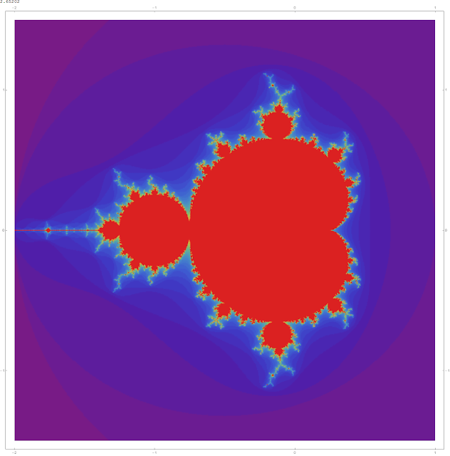
Start with a couple of individual plots. I use ImageSize->Full so when you do this yourself a large image will automatically be generated. On my Dell Optiplex 900 these take 2.68 seconds each.

Timing[DensityPlot[mandelbrot[x+I y],{x,-2,1},{y,-1.5,1.5},ColorFunction->Hue,PlotPoints->200,Mesh->False,ImageSize->Full,FrameTicks->{{-2,-1,0,1},{-1,0,1}}]]//Column

 Timing[DensityPlot[mandelbrot[x+I y],{x,-2,1},{y,-1.5,1.5},ColorFunction->"Rainbow",PlotPoints->200,Mesh->False,ImageSize->Full,FrameTicks->{{-2,-1,0,1},{-1,0,1}}]]//Column

 I'm kind of curious about all the built-in ColorFunctions. Let's plot Mandelbrot sets using each of them. Here they are. I reverse the order since I like some of the ones at the end best.

colorFunctions=ColorData@"Gradients"

{AlpineColors,Aquamarine,ArmyColors,AtlanticColors,AuroraColors,AvocadoColors,BeachColors,BlueGreenYellow,BrassTones,BrightBands,BrownCyanTones,CandyColors,CherryTones,CMYKColors,CoffeeTones,DarkBands,DarkRainbow,DarkTerrain,DeepSeaColors,FallColors,FruitPunchColors,FuchsiaTones,GrayTones,GrayYellowTones,GreenBrownTerrain,GreenPinkTones,IslandColors,LakeColors,LightTemperatureMap,LightTerrain,MintColors,NeonColors,Pastel,PearlColors,PigeonTones,PlumColors,Rainbow,RedBlueTones,RedGreenSplit,RoseColors,RustTones,SandyTerrain,SiennaTones,SolarColors,SouthwestColors,StarryNightColors,SunsetColors,TemperatureMap,ThermometerColors,ValentineTones,WatermelonColors}

Length@colorFunctions

51

I'll make a Grid of them that will correspond to the Grid of the plots themselves so we can easily look up the ColorFunction of one we like by finding its name in the corresponding place in the Grid. Although each row will have 3 plots and 3 divides 51 evenly, by habit I use the syntax for Partition that would not drop an overhang of a ragged List (the empty List {} in the position of the padding argument).

Reverse@colorFunctions//Partition[#,3,3,1,{}]&//Grid

The iterator, predefined, in this Table iterates over all the ColorFunctions. Note you do not need to use the cumbersome {i, Length@colorFunctions} requiring the iterator to be a number.

Table[DensityPlot[mandelbrot[x+I y],{x,-2,1},{y,-1.5,1.5},ColorFunction->predefined,PlotPoints->200,Mesh->False,FrameTicks->{{-2,-1,0,1},{-1,0,1}},ImageSize->Medium],{predefined,Reverse@colorFunctions}]//Partition[#,3,3,1,{}]&//Grid

Recommended:

What I Gave Stephen Wolfram On His 50th Birthday

To celebrate the 25th anniversary of Mathematica's release, I will post some Mathematicana. I'll explain this chart more fully later but here is a précis. Stephen developed Mathematica in part so that he'd have a powerful tool with which to explore the targets of his curiosity. (And we benefit by having a powerful tool with which to explore the targets of our curiosity!) The principal result of his explorations is A New Kind of Science (NKS for short), during the writing of which,  thanks to Mathematica, he made "more discoveries than I ever thought possible" (NKS p 22).

Until recently the history of science and separately, mathematics, displayed the great theme of logical reductionism, by which I mean our success at reducing disparate phenomena to a relatively few postulates or axioms. Viz, physics, or mathematics. While Wolfram's key discovery was that a short sequence can generate unlimited complexity (NKS Ch 2) and while "short sequence" does imply reductionism, the unlimited complexity is anti-reductionistic. To expose the phenomena described by some short sequences we must compute them interminably. This chart, an attempt to place NKS in history, is what I gave Stephen on his birthday several years ago (click to enlarge).

The "flowstream" term is from the lectures of Andrew J. Galambos, a great, but largely unsung, philosopher. When I mentioned the concept of an intellectual flowstream to my friend Dave Waltz, he pointed me to the fascinating work of Eugene Garfield, notably the Web of Science.