How to Lose List Brackets in Mathematica

First, Apply, Sequence, ReplaceAll

There come times in every Mathematica user's life when the all-pervasive List brackets get in the way. Sometimes it's easy to redesign the function to accept the arguments in a List. Here are other solutions.

First

For a single element enclosed by brackets, you can use First to extract the element. In this example, since all Mathematica arithmetic functions are Listable (they will automatically Map over a List) we specify that the argument must be an Integer so the function will fail.

enclosed1={2};
Clear@function1;function1@x_Integer:=x^3;
function1@enclosed1

function1[{2}]

function1@First@enclosed1

8

Apply

First, see if you can use Apply @@ to apply a function to the contents of your List. Apply will replace the List head with your desired function and Evaluate it.

In[107]:=  Range@15
Out[107]=  {1,2,3,4,5,6,7,8,9,10,11,12,13,14,15}

In[108]:=  Plus@@%
Out[108]=  120

Here's a single filename that is unnecessarily surrounded by List brackets. It's a String, so we just Apply ToString to it. It then stands alone – no List brackets – but its Head is String.

FileNames[]

{TableFiredFibers-Control-CathodeOnly-0p644.txt}

ToString@@%141

TableFiredFibers-Control-CathodeOnly-0p644.txt

Head@%
String

FullForm@%%
"TableFiredFibers-Control-CathodeOnly-0p644.txt"

Sequence

Mathematica was designed as a list processing language in which the list is the fundamental data structure. Allan Newell's IPL (Information Processing Language) was the original prototype, after which John McCarthy coupled the list as a universal data structure with the lambda calculus and logic functions into the major programming language, LISP.

We can Apply Sequence to a List to replace List as the container (the Head). Here are two examples, first to a single List, then to a List of Lists.

In[115]:= Sequence@@{0,4}

Out[115]= Sequence[0,4]

In[119]:= Sequence@@{{0,1,1},{0,2},{0,1,3},{0,4}}

Out[119]= Sequence[{0,1,1},{0,2},{0,1,3},{0,4}]

FileNameJoin is the safe way to assemble filepaths in Mathematica since it knows your operating system syntax. However FileNameJoin only accepts a single-level List as its argument. To feed it a nested List, use Sequence instead of List as the Head of the inner List.

In[350]:= twoPathElements={"webPages","index.html"};

In[351]:= FileNameJoin@{$HomeDirectory,twoPathElements}

Out[351]= FileNameJoin[{C:\Users\kwcarlso,{webPages,index.html}}]

Since it didn't see a List of Strings (filepath names) as the correct argument types, FileNameJoin returned the input. Using Sequence solves this.

In[352]:= twoPathElements=Sequence["webPages","index.html"];

In[353]:= FileNameJoin@{$HomeDirectory,twoPathElements}

Out[353]= C:\Users\kwcarlso\webPages\index.html

The context of one function I use to illustrate Sequence is worth mentioning (but skip this to get to more usages of Sequence). I have digitally sampled a curve from the literature (a paper by Holsheimer from 1999) in the graphing program Origin. In other words, you can import an image, in this case a graph for which Holsheimer doesn't give either the underlying data or an equation, and repeatedly click on it to harvest {x,y} values. We captured 163 sample points on the solid curve below, which is a vast improvement on the antiquated method of using a straightedge to pick up x and y values off the axes.

With that many sample points, finding the x value closest to the one desired is a reasonable alternative to fitting a curve and applying the fit equation to values you wish to interpolate or extrapolate.

So this is a function to find the nearest x value (a neuron axon diameter, fiberDiameter) to one for which we want to know the threshold as determined by Holsheimer (which is the y-value retrieved). The problem is Nearest returns values in List brackets, which don't match the un-bracketed x values in the List of data. Applying Sequence to the result of Nearest feeds the unbracketed value to Cases, which then performs the match.

Clear@diameterThreshold; diameterThreshold[fiberDiameter_, fiberThresholdSourceData_:holsheimerData1999] := Cases[fiberThresholdSourceData, {x_, y_} /; x == Sequence@@Nearest[fiberThresholdSourceData[[All, 1]], fiberDiameter] ]

So in sum this function says: Clear the function name (which I do habitually at the start of a function definition to prevent accidentally testing a previous version as I revise it). Then define it as the Cases in the source data file (fiberThresholdSourceData--default to the holsheimerData1999 file unless I specify another file) such that ( /; ) the x-value is Nearest to the fiberDiameter parameter I give it.

ReplaceAll

Here is a third way using rule patterns.

In[128]:= {{0,1,1},{0,2},{0,1,3},{0,4}}/. List[a__] ->a

Out[128]= Sequence[{0,1,1},{0,2},{0,1,3},{0,4}]

Mathematica Keyboard Shortcuts

Keyboard Shortcuts and Handy Short Commands

Here are some useful and lesser-known keyboard shortcuts. In terms of saving time, rather than using brackets for single-argument functions, use Prefix: function@argument.

Likewise, nesting functions with increasingly distal matched brackets is difficult to read, increases programming time, and obstructs you highlighting what you feel is important in the function. Use Postfix-style with pure Functions like this:

dataFiles[[1]]//Rest//Flatten//Length;

dataFilesDifferences//Chop[#,10^-4]&//Union/@#&//ListPlot/@#&//Partition[#,3]&//Grid

As advocated in my 2007 User Conference talk (also here), a "Functional-Procedural Fusion" elegantly represents deeply nested functions in a readable manner. If you do use deeply nested functions, multiple-clicking the Head of an Expression will select its brackets.

Ctrl+F6          Switch between open Mathematica notebooks
F12                Toggle current notebook to and from full screen

Ctrl+Shift+K  After a function name gives you a template for the simplest form of the function

Ctrl+K            After a function name gives a drop-down listbox with autocompletions of the function

?*name*         As in "?*Plot*" lists all Mathematica functions with Plot in their name. You can then click on them to get quick help text.

?Global`*       Lists all Names created in current Mathematica session

F1                  Search Help for expression to left of cursor

Shift + F1      Open new instance of Help browser. Do scratchpad calcs in Help rather than opening a new Notebook. They're automatically cleaned up when you go to a new Help topic.

Alt+.              Interrupt a computation. If it doesn't work, do Evaluation/Quit Kernel.
Shift+Alt+.    Remove a selected computation from the Evaluation queue. This is handy when you have a long computation running, start another one, and want to abort that one without aborting the one that is running.

Rather than using palettes, just learn keyboard shortcuts for the symbols you use frequently, for example:

esc+[character}+esc  E.g. to give the Greek letter corresponding to the keyboard character
Ctrl+6             Superscript
Ctrl+-              Subscript
Alt+7              Format cell as plain text
Alt+6              Format cell as Subsubsection
Alt+5              Format cell as Subsection

%+Out line    As: %127. Refers to output line #127. Same as Out@127 or Out[127] but more concise. I use this frequently for a temporary variable name but if it turns out I need a more permanent mnemonic name I just create one: newName = %127. I use %, %%, or %2 only for very temporary "scratchpad" calcs.

Ctrl+L            Copy input cell from the one just above
Ctrl+Shift+L   Copy output cell from the one just above, into new input cell. An alternative is to just start typing in the Output cell and Mathematica automatically creates a new Input cell with those contents.

Clear@%127  Removes from memory some huge expression you created or imported in In[127].
ClearAll["Global`*"] and Remove["Global`*"] Clears or Removes all values from variables you created in the current session. If it comes to that, I usually kill the kernel though (Evaluation/Quit Kernel).

filePath="C:\\directory1\\directory2"; FileNameSetter@Dynamic@filePath

Gives you a in-Notebook button to click to navigate and select a filename or directory to which to Set filePath. Giving filePath an initial value before evaluating FileNameSetter takes you to that value (e.g. a directory) when you click the button. Using Dynamic lets you click the button over and over to re-Set filePath.

CreateDocument@expression Opens a new Mathematica notebook with expression in it. Expression can be an imported document.

Mathematica Plot: Using Table to See Numerical Values

Plot with Table to See Numerical Values

We saw how to use Table to generate sample points for a ListPlot, and how to compare your own sample to Plot showing its mesh points. Here is the converse usage, using Plot to graph a function and then Table to see it numerically. We'll start with a simple sine curve.

To see numerical values, I click Control+L to regenerate the input, replace "Plot" with "Table", and specify a third argument for the iterator to give the sampling frequency. The Postfix function N tells Mathematica to give us decimal output instead of its default, exact fractional values.

In[314]:= Table[{x, Sin@x // N}, {x, 0, 2 Pi, Pi/4}] // TableForm

Let's look at a more complicated example with two decay curves that are identical except for their asymptotes, which are 0 for decay1 and 0.7 for decay 2 (shown in the Plot).

In[347]:= Clear@decay1; decay1@d_ := (q/d) + 0.7; q = .2;

In[348]:= Clear@decay2; decay2@d_ := (q/d); q = .2;

In[363]:= Plot[{decay1@d, decay2@d}, {d, .1, 4}, PlotRange -> {Automatic, {0, 3}}]

When you need to keep track of three or more columns, TableHeadings can be helpful. Here we say no row headings, but three column headings.

Table[{d, decay1@d, decay2@d}, {d, .1, 1.2, .1}] // 

 TableForm[#, TableHeadings -> {None, {"d", "decay1@d", "decay2@d"}}] &

Mathematica Plot: Options Overview

Plot Has over 80 Options to Control its Behavior


Here is a Plot of two curves where we use Plot options to add a Frame, tick marks to the left and right y-axes, but to the bottom x-axis only, and to Plot the full -y-range instead of leaving out extreme values.

Plot[Tooltip@{Sin@x, x Sin@x}, {x, 0, 20}, Frame -> True,
 FrameTicks -> {{Automatic, All}, {Automatic, None}}, PlotRange -> Full]

You can ask Mathematica for all the available Options for a function with Options@function. When you do, Mathematica tells you their default values as well.

Options@Plot // Partition[#, 3,3,1,{}] & // TableForm

The Partition syntax may look a little complicated, but is explained in Capturing the Remnant of a Partitioned List. It says: "Partition the list into sublists of length 3, take them in blocks of 3 (i.e. do not overlap them), start the first element of the first list at position 1 of the first sublist (at the beginning), and do not pad the last uneven list (i.e. pad it with the empty set)." While Plot has 57 Options, which divide evenly by 3, the partition syntax will work if Plot has a non-divisible-by-3 number of Options in the future.

I thank a diligent reader, Murta, for suggesting this correction to my original post.

Plotting Constant Functions

Plotting Constant Functions


You may want to plot a constant, for instance to combine with another plot. To do this you specify the constant without a function and the domain within which you want to plot the function.

Plot[5, {x, 0, 5}]

Suppose you want to plot a constant x value for all y. That's not a function and Plot won't work. For instance, you may want to plot a vertical asymptote and while Mathematica will plot vertical asymptotes for some functions (see the plot for Tan@x in tutorial/Basic Plotting), it may not for all. Here is one method. Note that any number followed by pure Function "&" makes a constant Function for that number's value. In other words, the constant Function yields the constant no matter what number it is applied to.

4.5 & /@ {5, 28.6, Pi, E}

{4.5, 4.5, 4.5, 4.5}


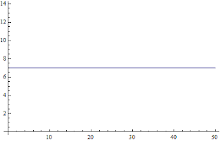
Here we use the constant pure Function to create the x-values as just shown. Thread with List creates the 50 pairs of y-values for x = 7.

Thread[List[7 & /@ Range[0, 50], Range[0, 50]]] // Short

{{7,0},{7,1},{7,2},{7,3},{7,4},{7,5},{7,6},{7,7},<<35>>,{7,43},{7,44},{7,45},{7,46},{7,47},{7,48},{7,49},{7,50}}

ListLinePlot[Thread[List[7 & /@ Range[0, 50], Range[0, 50]]]]

And so this is also a way to plot a constant y value by using the constant Function for the range instead of the domain.

ListLinePlot[Thread[List[Range[0, 50], 7 & /@ Range[0, 50]]]]

Mathematica Plot: Plotting More than One Function

Using Plot to Plot More than One Function


It is often useful to Plot different function parameter values and compare them. Just give Plot a list of functions with the parameter values you wish to compare and it will Plot them together without your having to use Show. Let us use the function defined in Basic Plotting:


f[x_, t_] := x^t;


You can use Table to automate the parameter sweep, but pre-generate the sweep functions or (for reasons I don't understand) Plot won't automatically color-code them.

In[278]:= sweepFunctionTable = Table[f[x, t], {x, 2, 5}]

Out[278]= {2^t, 3^t, 4^t, 5^t}

In[279]:= Plot[sweepFunctionTable, {t, 0, 5}]

Plot with Tooltip to Identify the Plots

Sometimes you can lose track of which function is which when plotting several function together. Plot helps by color-coding them. But adding Tooltip labels is another technique. Let's compare the three functions Sin x, Cos x, and Sin x + Cos x. You will need to Plot this yourself in a Notebook to mouseover and see the tooltips that label each curve with the three function names ("Sin@x", "Cos@x", "Cos@x + Sin@x").

Plot[Tooltip@{Sin@x, Cos@x, Cos@x + Sin@x}, {x, -3 Pi, 3 Pi}]

Now let's specify that the tick marks should be labeled in radians:

Plot[Tooltip@{Sin@x, Cos@x, Cos@x + Sin@x}, {x, -3 Pi, 3 Pi},
 Ticks -> {{-3 Pi, -2 Pi, -Pi, 0, Pi, 2 Pi, 3 Pi}, Automatic}]

Mathematica Plot - Basic Plotting

Plot

For starters, be aware that Mathematica's data plotting functionality is extensive and there are a variety of Plot functions. Using Information "?" with the wildcard characters "*" shows all functions that include "Plot". I won't show them here, but you can execute the command if you wish to see them.

?*Plot*

Basic Plotting

Let's say you have a function and you want to understand its behavior. We'll do a simple one.

In[238]:= y == x^n // TraditionalForm

Out[238]//TraditionalForm= y==x^n

Let's start by generating a few sample points of the function and plotting them.  You might think in the age of computers we can dispense with plotting sample points and just let Plot do the job. But when Plot fails to give you output and you don't know why, one measure is to go ahead and plot a few sample points by hand and compare them to what Plot is doing. So let's generate the sample points the easy way with Table. We Clear the function name, define the function, give x a value of 2, and use Table to sample the domain from -5 to 5 in increments of 0.5.

In[249]:= Clear@f; f[x_, t_] := x^t;

In[250]:= samplePoints = Table[f[2, t], {t, -5, 5, .5}]

Out[250]= {0.03125, 0.0441942, 0.0625, 0.0883883, 0.125, 0.176777, 0.25, 0.353553, 0.5, \
0.707107, 1., 1.41421, 2., 2.82843, 4., 5.65685, 8., 11.3137, 16., 22.6274, \
32.}

Now we plot these values using ListPlot. Ignore for now the x-tick points, which are just the number of the data point in the List.

In[242]:= plot1 = ListPlot@samplePoints

To better visualize the function, it's often helpful to connect the sample points. We use ListLinePlot. Another way is to use ListPlot's option, Joined -> True). If you look closely, you can see that the sample points are joined by line segments; our plot is not a continuous curve. Again, ignore the abscissa values.

plot2 = ListLinePlot@samplePoints

If we wished, we could combine the plots with Show--one of the most commonly-used plot techniques.

Show[plot1, plot2]

And this is similar to what Plot does--sampling a function and plotting the connected sample points--but of course in a much more sophisticated way. For one thing, Plot samples more frequently where it thinks it might need to, such as where the value of the function changes more frequently, maybe with several tries, and automatically connects the sample points in a continuous curve. Using Plot the x-axis values are correctly labeled.

Plot[f[2, t], {t, -5, 5}]

But notice that Plot is not showing the full domain and range that we asked for. By default it tries to, in effect, show the most important part of a function by excluding what it thinks might be outliers. Two options allow you to override this behavior. PlotRange->Full tells Plot to not clip the y-axis. PlotRange->All tells Plot to include all domain points and their y-values. I usually use PlotRange->All.

Plot[f[2, t], {t, -5, 5}, PlotRange -> All]

If you wish, reveal the sample points with the Option, Mesh->All. When you don't understand what Plot is doing, revealing the Mesh is a good first step. And then as I said above, you can compare Plot's sample points to yours, which might illuminate what's going on. There are more Mesh options to allow you to control how Plot uses its sample points.

Plot[f[2, t], {t, -5, 5}, Mesh -> All, PlotRange -> All]

Next: Using Plot to Plot More than One Function