Apply a List of Functions to a Corresponding List of Arguments

Here are two ways to apply a List of functions to a List of arguments. The first method, from Maeder, uses Inner. Note the use of a purely symbolic example to reveal what Inner is doing.

Inner[#@#2&,{f1,f2,f3,f4},{arg1,arg2,arg3,arg4},List]

{f1[arg1],f2[arg2],f3[arg3],f4[arg4]}

In #1@# &, Slot1 (#1 or abbreviated #) pulls an argument from the first List, which are the functions, and Slot2 (#2 where you do need the "2") pulls an argument from the second List, which are the arguments.

If you wanted to apply a second function, g, to the results rather than just listing them, Inner provides for that:

Inner[#@#2&,{f1,f2,f3,f4},{arg1,arg2,arg3,arg4},g]

g[f1[arg1],f2[arg2],f3[arg3],f4[arg4]]

The second method, from my Mathematica teacher Harry Calkins, uses MapThread, which requires wrapping the function List and the argument List together in a List:

(arguments={{a,b,c},{d,e,f},{r,s,t},{u,v,w}});

(functions={3 #&,3+#&,#/2&,Plus@@@Partition[#,2,1,{1,1},#]&});

He gave an example using some built-in functions and structured the functions and arguments in matrices.By enclosing the assignments in parentheses he showed them as matrices without inadvertently making the assignment to the MatrixForm-formatted List.

arguments//MatrixForm
functions//MatrixForm

(results=MapThread[#1@#2&,{functions,arguments}])//MatrixForm

String Processing: Validate Email Address Format, Part 1

Here are three approaches to predicates validating that an email address has an "@" sign and a period ".". A true email address validator is much more complicated, so these functions are merely to illustrate some String processing techniques. That said, I did use the first approach to validate thousands of email addresses and flush out bad ones.

The first predicate uses StringMatchQ and the essential idea is to give StringMatchQ a String pattern representing:

1. An "@" wildcard for at least one but an unknown number of characters
2. Followed by the "@" sign as used in an email address to separate localpart from domain
3. Followed by the wildcard again
4. Followed by the period "." used to separate the mail server name from the top-level domain
5. Followed by the wildcard

Note that an asterisk wildcard ("*") would not be suitable since each position in the pattern has at least one character.

The first variation illustrates the use of Verbatim, which tells Mathematica to treat the middle "@" sign as an "@" sign  (read it "verbatim") and not as a pattern wildcard.

Clear@emailAddressQ1;emailAddressQ1@aString_String:=StringMatchQ[aString,"@"~~Verbatim@"@"~~"@.@"]

The second variation of StringMatchQ does the same thing but more concisely, using a double backslash. The first backslash tells Mathematica to treat the second one as an 'escape' character, which then tell Mathematica to treat the "@" sign as an "@" sign and not as a wildcard.

Clear@emailAddressQ1a;emailAddressQ1a@aString_String:=StringMatchQ[aString,"*\\@*.*"]

The second basic approach uses StringContainsQ to detect the presence of the "@" sign and period "." in the address. Since it doesn't require additional characters in the correct positions as does the first approach, it is not as good a validator.

Clear@emailAddressQ2;emailAddressQ2@aString_String:=StringContainsQ[aString,"@"]&&StringContainsQ[aString,"."]

The third approach uses StringFreeQ to see if the address has no "@" sign and period ".", and some logic, and suffers the same limitation as the second approach.

Clear@emailAddressQ3;emailAddressQ3@aString_String:=Not[StringFreeQ[aString,"@"]&&StringFreeQ[aString,"."]]

Test Cases

The test cases are 1) valid email format, 2) missing "@" sign, 3) missing "." and 4) missing both "@" and ".".

testCases={"abc@dwxy.anything","abcdwxy.anything","abc@dwxyanything","abcdwxyanything"};

emailAddressQ1/@testCases

{True,False,False,False}

emailAddressQ1a/@testCases

{True,False,False,False}

emailAddressQ2/@testCases

{True,False,False,False}

emailAddressQ3/@testCases

{True,True,True,False}

Aha! The test cases flushed out a logic error. The way the emailAddressQ3 function is written with the AND (&&) conjunction between the two clauses, only if both StringMatchQ tests are FALSE will AND return FALSE and be negated by NOT into TRUE. We need to change the AND to OR so that if either "@" or "." are missing, the OR returns TRUE and is negated by NOT into FALSE.

Clear@emailAddressQ4;emailAddressQ4@aString_String:=Not[StringFreeQ[aString,"@"]||StringFreeQ[aString,"."]]

emailAddressQ4/@testCases

{True,False,False,False}

Grid - Partition - Identify Primes with Formatting

Starting with an example from Mangano, Mathematica Cookbook, and the Doc Center, here are examples of using Partition with Grid and formatting to highlight the values of interest.

Grid@Partition[If[PrimeQ@#,Framed[#,FrameStyle->Red],#]&/@Range@200,20]

Grid@Partition[If[PrimeQ@#,Style[#,FontColor->Red],#]&/@Range@200,20]

Grid@Partition[If[PrimeQ@#,Style[#,FontColor->Red,FontWeight->Bold],Style[#,FontColor->Gray]]&/@Range@200,20]

This sets up a clickable square from which you can interactively choose a color.

Clear@highlightColor;ColorSetter@Dynamic@highlightColor

Then the selected color is used here:

Grid@Partition[If[PrimeQ@#,Style[#,FontColor->highlightColor,FontSize->16,FontWeight->Bold],Style[#,FontColor->Gray]]&/@Range@200,20]

Grid@Partition[If[!PrimeQ@#,Style[#,FontColor->White],#]&/@Range@200,20]

Change the Partition from 20 to 10 to accommodate larger numbers.

Grid@Partition[If[!PrimeQ@#,Style[#,FontColor->White],#]&/@Range[500000,500200],10]

Run Wolfram BenchmarkReport to Test Your Computer's Peformance

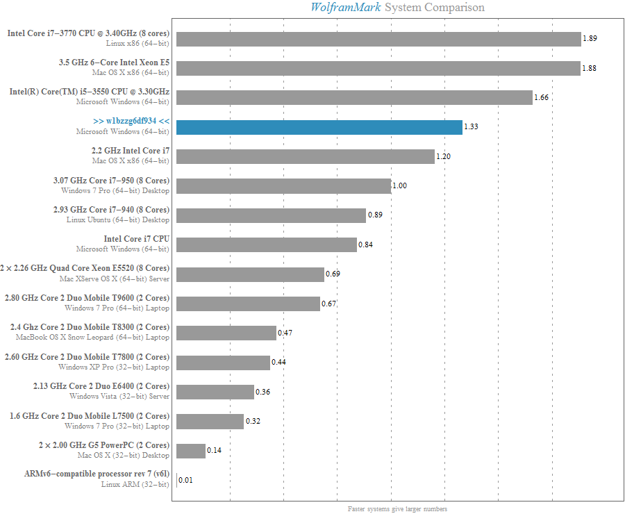
This is kind of neat. The report will compare your computer to a garden variety of others based on some benchmark tests. Your computer's results will be highlighted in blue. Interestingly I found that our more expensive and supposedly fastest computer ranked 7th compared to our standard desktops, which ranked 4th.

The actual tests and code for them are very interesting — see the bottom of the report.

?BenchmarkReport[]

BenchmarkReport[] runs the WolframMark benchmark and produces a report in a separate notebook comparing this system to a selection of reference systems.

BenchmarkReport[system1,system2, ..., data1,data2,...] produces a custom report comparing the specified systems from $BenchmarkSystems and the specified data returned from Benchmark. >>

Needs@"Benchmarking`";
BenchmarkReport[]

WolframMark Benchmark Report

Machine Name: w1bzzg6df934
System: Microsoft Windows (64-bit)
Date: December 3, 2015
Mathematica Version: 10.2.0
Benchmark Result: 1.33

WolframMark Results

WolframMark Sources

Test 1: Data Fitting

Module[{data},AbsoluteTiming[data=Flatten[Table[{x,y,z,Log[120 x]-Abs[Cos[z/300]/(140 y)]},{x,0.2`,10,0.22`},{y,0.2`,10,0.22`},{z,0.2`,10,0.22`}],2];FindFit[data,Log[a x]-Abs[Cos[b z]/(c y)],{a,b,c},{x,y,z},AccuracyGoal->6];]]

Test 2: Digits of Pi

AbsoluteTiming[N[\[Pi],1000000];]

Test 3: Discrete Fourier Transform

Module[{data},AbsoluteTiming[SeedRandom[1];data=RandomReal[{},{1200000}];Do[Fourier[data],{11}]]]

Test 4: Eigenvalues of a Matrix

Module[{a,b,m},AbsoluteTiming[SeedRandom[1];a=RandomReal[{},{420,420}];b=DiagonalMatrix[RandomReal[{},{420}]];m=a.b.Inverse[a];Do[Eigenvalues[m],{6}]]]

Test 5: Elementary Functions

Module[{m1,m2},AbsoluteTiming[SeedRandom[1];m1=RandomReal[{},{2.2`*^6}];m2=RandomReal[{},{2.2`*^6}];Do[Exp[m1];Sin[m1];ArcTan[m1,m2],{30}]]]

Test 6: Gamma Function

Module[{a},AbsoluteTiming[SeedRandom[1];a=RandomInteger[{80000,90000},{55}];Gamma[a]]]

Test 7: Large Integer Multiplication

Module[{a},AbsoluteTiming[SeedRandom[1];a=RandomInteger[{10^1100000,10^(1100000+1)},{}];Do[a (a+1),{20}]]]

Test 8: Matrix Arithmetic

Module[{m},AbsoluteTiming[SeedRandom[1];m=RandomReal[{},{840,840}];Do[(1.` +0.5` m)^127,{50}];]]

Test 9: Matrix Multiplication

Module[{m1,m2},AbsoluteTiming[SeedRandom[1];m1=RandomReal[{},{1050,1050}];m2=RandomReal[{},{1050,1050}];Do[m1.m2,{12}]]]

Test 10: Matrix Transpose

Module[{m},AbsoluteTiming[SeedRandom[1];m=RandomReal[{},{2070,2070}];Do[Transpose[m],{40}]]]

Test 11: Numerical Integration

AbsoluteTiming[NIntegrate[Sin[x^2+y^2],{x,-(2.6` \[Pi]),2.6` \[Pi]},{y,-(2.6` \[Pi]),2.6` \[Pi]}];]

Test 12: Polynomial Expansion

AbsoluteTiming[Expand[Times@@Table[(c+x)^3,{c,350}]];]

Test 13: Random Number Sort

Module[{a},AbsoluteTiming[SeedRandom[1];a=RandomInteger[{1,50000},{520000}];Do[Sort[a],{15}]]]

Test 14: Singular Value Decomposition

Module[{m},AbsoluteTiming[SeedRandom[1];m=RandomReal[{},{860,860}];Do[SingularValueDecomposition[m],{2}]]]

Test 15: Solving a Linear System

Module[{m,v},AbsoluteTiming[SeedRandom[1];m=RandomReal[{},{1150,1150}];v=RandomReal[{},{1150}];Do[LinearSolve[m,v],{16}]]]

The Basics of Slot (#) in Pure Functions

Pure Function, as it's called, such as Function[x, x^2] that yields x² or the beautiful shorthand, #^2&, is extremely useful in Mathematica:

1. For one-time functions
2. As an argument in many functional-style commands such as Map, Nest, Fold, Select, Count, etc
3. In the extended Postfix style of programming I developed to eliminate hard-to-read nested functions
4. In predicates including those used for argument type-checking: _?(# <= 1 &)
5. In the general pattern-matching predicate MatchQ
6. And the new use in Associations in version 10

Slot must be used with the pure Function operator &. They are designed to be the Head of a function:

#1&[a,b,c]

a

When you use the Postfix style just remember that Postfix causes the ampersand abbreviation for Function to wrap around an entire expression preceding it. Thus it has a low precedence of 90; here are its neighbors:

Precedence/@{Set,Postfix,Colon,Function,TimesBy,Rule}

{40.,70.,80.,90.,100.,120.}

It can be confusing if there are nested used of Function, but using that principle, you can figure it out.

Important: What trips up beginners is using Slot with Mathematica's universal container, List. This doesn't work:

#1&{a,b,c}

{a (#1&),b (#1&),c (#1&)}

There are several solutions. Using Apply (@@) will return a Sequence:

args=##&@@{a,b,c,d}

Sequence[a,b,c,d]

A Sequence is a list designed to be fed to any function:

func@args

func[a,b,c,d]

You can wrap SlotSequence in List so it returns a List:

{##}&[a,b,c,d]

{a,b,c,d}

Here are typical uses with Function as the Head or using Apply. Note that you cannot use negative position numbers with Slot or SlotSequence since that would conflict with using Subtract in pure Functions (like #-2&).

"First" (the default position argument for Slot is 1 so you don't need to specify it with "#1")

#&@@{a,b,c}

a

Return the first two arguments:

{#,#2}&@@{1,2,3,4}

{1,2}

Return all arguments:  ## is SlotSequence, which returns a Sequence, which is designed to be given to any function as its argument list.

##&[a,b,c,d]

Sequence[a, b, c, d]

{##}&[a,b,c,d]

{a, b, c, d}

##&@@@[a,b,c,d]

{a, b, c, d}

Return the first and fourth arguments:

{#,#4}&@@{1,2,3,4}

{1,4}

"Rest": Return the 2nd argument to the last:

{##2}&[a,b,c,d]


Sequence[b,c,d]

As of version 10, there is an interesting new usage for Slot with Associations. Slot suffixed with any Key (name) of an Association will automatically return the Value associated with the Key.

cityPopulationAssociation=Association["Tokyo"->"37 million","Jakarta"->"26 million","Seoul"->"17 million","Delhi"->"22 million","Shanghai"->"21 million"];

#Delhi&@cityPopulationAssociation

22 million

Estimate Pi Using Monte Carlo Sampling

A classic use of the Monte Carlo random sampling technique is to estimate Pi. It's very simple.

1. We construct a square by randomly selecting point in the interval (-1, 1).

2. We select a subset of points that satisfy the predicate that places them on or within the unit circle:

x^2 + y^2 < =1.

3. The area of the square extending from -1 to 1 is 2^2 = 4. The area of the unit circle is 1 (Pi*r^2 = Pi*1^2). Therefore we multiply the ratio of the number of points lying within the unit circle divided by the number of points within the square by 4.

Here is an implementation. Below that is an implementation I found on the web that shows how newbies to Mathematica may transfer inefficient coding techniques from other languages to Mathematica.

Clear@circleRegionMonteCarlo;circleRegionMonteCarlo[numberSamplePoints_Integer]:=Module[{samplePoints=RandomReal[{-1,1},{numberSamplePoints,2}],
areaOfCirclePoints},

(* Select points within the unit circle using the parametric equation for a circle *)
areaOfCirclePoints=Select[samplePoints,First@#^2+Last@#^2<=1&];

Print@StringForm["Approximation to Pi using `` sample points is ``.",numberSamplePoints,4*Length@areaOfCirclePoints/numberSamplePoints//N];

If[numberSamplePoints<50001,ListPlot[areaOfCirclePoints,AspectRatio->Automatic]]
]

circleRegionMonteCarlo[50000]

Approximation to Pi using 50000 sample points is 3.14104`.

This represents an obsolete coding technique: 1) initializing the Pin (points inside the circle) and Pout (points outside the circle) arrays, 2) the For loop calling named random variable functions, 3) testing the distance predicate in the loop instead of all at once as is typical in functional programming, 4) having to take the Length of Pin and Pout in the loop (obviously you don't need to test the Length every time anyway), and 5) using Return instead of just leaving off the semi-colon after approx, are all obsolete techniques.

MonteCarloPi[n_]:=Module[{d,i},
n=n0;
Pin=Pout={};
For[i=1,i<=n,i++,
x=RandomReal[];
y=RandomReal[];
d=x^2+y^2;
If[d<=1, Pin=Append[Pin,{x,y}],Pout=Append[Pout,{x,y}]  ];
n=Length@Pin;
m=Length@Pout;
\[Rho]=m/n;
approx=4.0;]
Return@approx

]

How It Works: Union

Here is a recursive version of the set-theoretic function, Union, which returns the common elements of two or more sets (represented as Lists in Mathematica).

There are two base cases: 1) The union of any set with the empty set is the set itself, and 2) The union of any set with a single element set is the single element set appended to the other set. The recursive case is: 3) The union of any two Lists is the union of the first List with the First element of the second List (i.e. the single element base case), which, calling itself, recurses down the Rest of the second List until it hits the empty set base case (an empty List), at which point it unwinds back out to produce the overall union.

Union produces a set of unique elements  — no duplicates — so we need to de-dupe the List. An easy way to do that is Sort it and use a replacement Rule (we could also use the built-in DeleteDuplicates or How It Works: DeleteDuplicates).

I show two ways to control the Precedence of the abbreviate operators for ReplaceRepeated vs Postfix. Since with Precedence of 110 ReplaceRepeated is a little 'stickier' than Postfix at 70 Sort will stick to the ReplaceRepeated function unless we do something. So we can either enclose the compound function in parentheses before applying ReplaceRepeated as in the 2^nd base case or we can use Postfix with Slot (#) and pure Function (&) as typical in my extended Postfix syntax as in the recursive case.

Clear@myUnion;

myUnion[list1_List,{}]:=list1; (* 1st base case *)

myUnion[list1_List,element_]:=(If[MemberQ[list1,element],list1,list1/.{x___}->{x,element}] //Sort)//.{a___,b_,b_,c___}->{a,b,c}(* 2nd base case *)

myUnion[list1_List,list2_List]:=Module[{union},union=myUnion[myUnion[list1,First@list2],Rest@list2]//Sort//#//.{a___,b_,b_,c___}->{a,b,c}&
] (* recursive case *)


myUnion[{1,2,3,4},{}]

{1,2,3,4}

myUnion[{1,2,3,4},5]

{1,2,3,4,5}

myUnion[{1,2,3,4},2]

{1,2,3,4}

This shows the need to add a delete duplicates function:

myUnion[{1,2,2,3},2]

{1,2,2,3}

A simple replacement Rule does the job, but use ReplaceRepeated or only the first instance of a duplicate will be replaced:

{1,2,2,3,4,4}/.{a___,b_,b_,c___}->{a,b,c}

{1,2,3,4,4}

{4,4,1,3,3,2,2}//.{a___,b_,b_,c___}->{a,b,c}

This works without the delete duplicates function.

myUnion[{1,2,3,4},{3,4,5,6}]

{1,2,3,4,5,6}

But this would fail without it. First without delete duplicates.

myUnion[{1,2,2,3,4},{3,4,5}]

{1,2,2,3,4,5}

And now with delete duplicates.

myUnion[{1,2,2,3,4},{3,4,5}]

{1,2,3,4,5}

And the base case.

myUnion[{3,2,1,2,2,3},3]

{1,2,3}

And the recursive case.

myUnion[{1,2},{2,3,4}]

{1,2,3,4}

How to See the Equivalence of Select and Cases

MatchQ and PatternTest Equate Cases and Select

Select and Cases are essential Mathematica filtering functions. Select filters expressions, usually Lists, with predicates, such as ones that end with Q (evaluate ?*Q to see them) or those that don't, such as Greater, Less, and others that I list here. Cases uses patterns such as testing for a Head (e.g. _Integer) or a more general pattern (e.g. for a 2-element List, {x_,y_}.

Cases and Select are equivalent and a versatile Mathematica programmer knows how to use either one in any circumstance according to the need of the moment. The keys to seeing their equivalence are MatchQ, which translates a pattern into a predicate, and PatternTest (_?test), which translates a predicate into a pattern.

MatchQ[4.1,_Real]

True

MatchQ[{2,2.1},{_Integer,_Real}]

True

Thus you can take any usage of Cases and translate it into Select.

Cases[{a,4,4.2,6,7.5,8},x_Integer/;x>4]

{6,8}

integerGreaterThan4Q@n_:=MatchQ[n,_Integer&&n>4];

Select[{a,4,4.2,6,7.5,8},integerGreaterThan4Q]

{6,8}

And you can take any usage of Select and translate it into Cases.

Select[{1,2,4,7,6,2},EvenQ]

{2,4,6,2}

Cases[{1,2,4,7,6,2},_?EvenQ]

{2,4,6,2}

If we built our own predicate for EvenQ using MatchQ, it works the same way.

Select[{1,2,3,4},MatchQ[#/2,_Integer]&]

{2,4}

However note the need for parentheses around the test, which is often the case with PatternTest - the no parens usage fails.

Cases[{1,2,3,4},_?(MatchQ[#/2,_Integer]&)]

{2,4}

Cases[{1,2,3,4},_?MatchQ[#/2,_Integer]&]

{}

The reason is that Blank and PatternTest both have a higher Precedence ('stickiness') than Function, and so they stick together and PatternTest ends up inside the pure Function instead of using the pure Function as the pattern test. You don't need to worry about that — just as a rule of thumb put parens around any 'homemade' test.

Precedence/@{PatternTest,Blank,Function}

{680.,730.,90.}

The Q Predicates

This is a handy way to use Partition, especially using {} so a final short sublist won't be dropped from a 'ragged' List. The syntax says

Partition[list, sublist length, offset length, start Position, padding]

and here means divide the List into Partitions of length 4, moving the window that same length 4 with each Partition so there is no overlap, start the List at Position 1,  and the empty set {} for padding tells Partition to return the final sublist even if it's shorter than what is specified by the 2nd argument, and don't pad that final short list. Evaluate this code in your Notebook:

Qpredicates=Names@"*Q";

Print@Length@Qpredicates;

Partition[Qpredicates,4,4,1,{}]//TableForm

Here's the same result in a List.

Names@"*Q"

{AcyclicGraphQ,AlgebraicIntegerQ,AlgebraicUnitQ,AntihermitianMatrixQ,AntisymmetricMatrixQ,ArgumentCountQ,ArrayQ,AssociationQ,AtomQ,BinaryImageQ,BipartiteGraphQ,BooleanQ,BoundaryMeshRegionQ,BoundedRegionQ,BusinessDayQ,ColorQ,CompatibleUnitQ,CompleteGraphQ,CompositeQ,ConnectedGraphQ,ConstantRegionQ,ContinuousTimeModelQ,ControllableModelQ,CoprimeQ,DateObjectQ,DaylightQ,DayMatchQ,DeviceOpenQ,DiagonalizableMatrixQ,DigitQ,DirectedGraphQ,DirectoryQ,DiscreteTimeModelQ,DisjointQ,DispatchQ,DistributionParameterQ,DuplicateFreeQ,EdgeCoverQ,EdgeQ,EllipticNomeQ,EmptyGraphQ,EulerianGraphQ,EvenQ,ExactNumberQ,FileExistsQ,firedQ,FreeQ,GeoWithinQ,GraphQ,GroupElementQ,HamiltonianGraphQ,HermitianMatrixQ,HypergeometricPFQ,ImageQ,IndefiniteMatrixQ,IndependentEdgeSetQ,IndependentVertexSetQ,InexactNumberQ,integerGreaterThan4Q,IntegerQ,IntersectingQ,IntervalMemberQ,InverseEllipticNomeQ,IrreduciblePolynomialQ,IsomorphicGraphQ,KEdgeConnectedGraphQ,KeyExistsQ,KeyFreeQ,KeyMemberQ,KnownUnitQ,KVertexConnectedGraphQ,LeapYearQ,LegendreQ,LetterQ,LinkConnectedQ,LinkReadyQ,ListQ,LoopFreeGraphQ,LowerCaseQ,MachineNumberQ,ManagedLibraryExpressionQ,MandelbrotSetMemberQ,MarcumQ,MatchLocalNameQ,MatchQ,MatrixQ,MemberQ,MeshRegionQ,MixedGraphQ,MultigraphQ,NameQ,NegativeDefiniteMatrixQ,NegativeSemidefiniteMatrixQ,NormalMatrixQ,NumberQ,NumericQ,ObservableModelQ,OddQ,OptionQ,OrderedQ,OrthogonalMatrixQ,OutputControllableModelQ,PartitionsQ,PathGraphQ,PermutationCyclesQ,PermutationListQ,PlanarGraphQ,PolynomialQ,PositiveDefiniteMatrixQ,PositiveSemidefiniteMatrixQ,PossibleZeroQ,PrimePowerQ,PrimeQ,ProcessParameterQ,QHypergeometricPFQ,QuadraticIrrationalQ,QuantityQ,RegionQ,RegularlySampledQ,RootOfUnityQ,SameQ,SatisfiableQ,ScheduledTaskActiveQ,SimpleGraphQ,SquareFreeQ,SquareMatrixQ,StringFreeQ,StringMatchQ,StringQ,SubsetQ,SymmetricMatrixQ,SyntaxQ,TautologyQ,TensorQ,TreeGraphQ,TrueQ,UnateQ,UndirectedGraphQ,UnitaryMatrixQ,UnsameQ,UpperCaseQ,URLExistsQ,ValueQ,VectorQ,VertexCoverQ,VertexQ,WeaklyConnectedGraphQ,WeightedGraphQ}

 

New in Mathematica 10: Associations as General-Purpose Associative Arrays

Associations are the most important data structure introduced in Mathematica in years. As the Guide says:

Along with lists, associations are fundamental constructs in the Wolfram Language. They associate keys with values, allowing highly efficient lookup and updating even with millions of elements. Associations provide generalizations of symbolically indexed lists, associative arrays, dictionaries, hashmaps, structs, and a variety of other powerful data structures. 

They of course will underlie databases and artificial intelligence data structures. They are intended to replace less structured expressions such as pairs in Lists or Rules. The code written for Association functions has been highly optimized for speed. I suspect that Associations are the core data structure of the Wolfram Alpha natural language processor, which is the front end for the curated data collections in Alpha, just as the Notebook is the front end for the kernel.

So when I needed a lookup table today I decided to try Associations. Here are some simple functions that define an axon's threshold in terms of the stimulating pulse seen at the axon, according to the Lapicque equation V_th = V_rh(1+τ_ch/pw).

(You don't need to understand these!)

absoluteRheobase@fiberDiameter_:=0.000589+0.01518 Exp[-fiberDiameter/2.3477]

chronaxie@fiberDiameter_:=102.764 +162.46744 Exp[-fiberDiameter/5.53435];

absoluteThreshold=.;absoluteThreshold[pulseWidth_,fiberDiameter_]:=Module[{},absoluteRheobase@fiberDiameter(1+chronaxie@fiberDiameter/pulseWidth)]

Now since fiber threshold is driven by their diameter and the pulse width of the stimulating pulse, we make sample tables of those. Esc + m + esc gives us the mu in microseconds and micrometers; no need to open a Palette.

pulseWidthTable50to500=Table[pw,{pw,100,500,100}] (* in μs *);

fiberDiameters1to15=Table[diameters,{diameters,5,10}] (* in μm *);

Now here is the function that creates the Associations. It took a bit of fiddling, but by making a Table of Rules in one step as should be done with good functional programming, it is then easy to Apply Association to the entire Table, simply replacing the Head, List, with Association, which converts the List of Rules into an Association. In the Table pulseWidth is the "i" iterator and fiberDiameter is the "j" iterator, and notice that we don't need to iterate numerically from 1 to Length@pulseWidthTable50to500, for example, we just directly iterate over the List itself, which is simpler.

absoluteThresholdTable=Association@@Table[Rule[{pulseWidth,fiberDiameter},absoluteThreshold[pulseWidth,fiberDiameter]],{pulseWidth,pulseWidthTable50to500},{fiberDiameter,fiberDiameters1to15}]

<|{100,5}->0.00642849,{100,6}->0.00455515,{100,7}->0.00337826,{100,8}->0.00263167,{100,9}->0.00215327,{100,10}->0.00184348,{200,5}->0.00441095,{200,6}->0.00316135,{200,7}->0.00236852,{200,8}->0.00186172,{200,9}->0.00153533,{200,10}->0.00132348,{300,5}->0.00373844,{300,6}->0.00269675,{300,7}->0.00203194,{300,8}->0.00160507,{300,9}->0.00132935,{300,10}->0.00115015,{400,5}->0.00340218,{400,6}->0.00246445,{400,7}->0.00186364,{400,8}->0.00147675,{400,9}->0.00122636,{400,10}->0.00106348,{500,5}->0.00320043,{500,6}->0.00232507,{500,7}->0.00176267,{500,8}->0.00139975,{500,9}->0.00116456,{500,10}->0.00101149|>

Here are several versions of lookup functions. The first one just uses the same syntax as we'd use to access elements of an associative array made with function@value, such as we'd construct with a memo function.

Clear@thresholdLookup; 
thresholdLookup[lookupTable_Association, pulseWidth_Integer, diameter_] := lookupTable@{pulseWidth, diameter}

absoluteThresholdTable@{100, 7}

0.00337826

Likely it's safer and more elegant to use the new Lookup function instead.

Clear@thresholdLookup2; 
thresholdLookup2[lookupTable_Association, pulseWidth_Integer, diameter_] := Lookup[lookupTable, {{pulseWidth, diameter}}]

thresholdLookup2[absoluteThresholdTable, 100, 7]

{0.00337826}

We see that using a List as the Key results in returning a List as the Value, like in solutions for equations returned by Solve, etc. So to access the Value we can use First@key to remove the List brackets, as we often do with solutions to equations.

Clear@thresholdLookup3; 
thresholdLookup3[lookupTable_Association, pulseWidth_Integer, diameter_] := Lookup[lookupTable, {{pulseWidth, diameter}}] // First

thresholdLookup3[absoluteThresholdTable, 100, 7]

0.00337826

Years ago I talked to Stephen Wolfram at an artificial life conference about artificial intelligence and his views were kind of naive. Things have changed. I expect that Mathematica and its Wolfram Language are headed inexorably toward large-scale AI applications,  approaching, and exceeding in some respects, human intelligence over the next two decades.

How to Find Memory Used in Computations

At some point you will need to — or just want to — push the limits of Mathematica and it may be helpful to measure memory consumed during a computation. Here are methods inspired by Wagon, Mathematica in Action (2nd ed., pp 431 et seq.). (See also Memory Management Tools.)

The first method is simple; store the initial MemoryInUse in a variable, do your calc, then subtract it from the current MemoryInUse.

currentMemory=MemoryInUse[];
{(MemoryInUse[]-currentMemory),Plus@@(1./Range@1000000)}

{1368,14.3927}

Second, suppose you want to monitor memory in several places in your code. Initialize the variable currentMemory, then sprinkle

Sow[-currentMemory+(currentMemory=MemoryInUse[])]

through your code like Print statements, and the enclosing Reap will cause each one to output the net memory consumed in bytes between the previous use and the current one. I say 'net' memory consumed because Mathematica is designed to optimize memory use and so clears memory in use every chance it gets. Following the pattern of Timing, I reverse the output to give the memory results first, then the function's output.

currentMemory=MemoryInUse[];
(*initialize s*); s=0;
Reap[Do[If[i<25,Sow[-currentMemory+(currentMemory=MemoryInUse[])]];s+=1./i,{i,1000}];s]//Reverse

{{{3016,11216,16,0,0,0,0,0,0,0,0,0,0,0,0,0,0,0,0,0,0,0,0,0}},7.48547}

Did you notice, as Wagon points out, that Do uses minimal memory during a calculation? It cleans up after every iteration.

Like Timing, this third method of checkMemory requires you to wrap your computation in checkMemory, access the result of your computation with First and if desired suppress the output with a semi-colon. Mimicking the structure of a built-in function is an example of a good programming technique. The designers of Mathematica are master programmers and they have created and debugged templates or paradigms of function structures. Often you can follow the structure of built-in functions to create sound ones of your own.

Clear@checkMemory;
checkMemory@computation_:=
Module[{computation1,preComputationMemory},
preComputationMemory=MemoryInUse[];Print["Memory in use at start is ",preComputationMemory];
computation1=computation;
memoryUsedInComputation=MemoryInUse[]-preComputationMemory;
Print["Memory in use at end is ",MemoryInUse[]];{memoryUsedInComputation,computation1}
]

Once it's done, this computation uses 32 bytes of memory and the result is 14.3927.

checkMemory[Sum[1./i,{i,1000000}]]

Memory in use at start is 31286024
Memory in use at end is 31286056
{32,14.3927}

We find the memory use with the function output for a small Table.

s1=0;checkMemory[Table[s1+=1./i,{i,10}]]

Memory in use at start is 31289472
Memory in use at end is 31289752
{280,{1.,1.5,1.83333,2.08333,2.28333,2.45,2.59286,2.71786,2.82897,2.92897}}

Then suppress output, with a semi-colon as is done in Timing, for a large Table.

checkMemory[s1=Table[1./i,{i,10^7}];]

Memory in use at start is 31340688
Memory in use at end is 111344696
{80003992,Null}

I left off the summation of the Table to show MemoryInUse during the calc. If we add Total, we see the max MemoryInUse reclaimed (-80,000,024 bytes).

Timing[checkMemory[s1=Table[1./i,{i,10^7}]//Total]]

Memory in use at start is 31359736
Memory in use at end is 31359864
{0.343202,{128,16.6953}}

Compare memory used in a Do loop. Pretty interesting!

Timing[s1=0;checkMemory[Do[s1+=1./i,{i,10^7}];s1]]

Memory in use at start is 31364400
Memory in use at end is 31364432
{10.296066,{32,16.6953}}

First@%/First@%%

30.0000

So there you have it, Do takes 30 times as long as the functional command Table[...]//Total, but uses a minute fraction of the latter's memory.

How to Query 11 Different Search Engines

You can query a search engine with URLFetch. For the URL you need a String that includes a standard prefix and a suffix that begins with something like "/?q=querykeywords". I have removed some unnecessary junk from most of the query Strings to make them as short and simple as possible.

There are several ways to functionally compose a query for a search engine. This one uses StringJoin. I use Which to handle the cases of 1) a single keyword, 2) multiple keywords, or 3) any other data type, which is an error. Using True as the third test in conditional statements is a standard way to handle 'all else' cases.

queryTemplateDuckDuckGo="https://duckduckgo.com/?q=";
keyword1="longevity";
keywords2={"machine","learning","algorithm"};

Clear@searchEngineQuery;
searchEngineQuery[searchEnginePrefix_String, keywords_] := 
 Module[{url},
  Which[
   Head@keywords === String, 
   url = StringJoin[searchEnginePrefix, keywords],
   Head@keywords === List, 
   url = StringJoin[searchEnginePrefix, 
     Table[i <> "+", {i, Most@keywords}], Last@keywords],
   True, Print@"Error: wrong data type."];
  Print@url;
  URLFetch@url
  ]

We test it on a single keyword (I omit the full output, which you can try at home).

searchEngineQuery@keyword1

https://duckduckgo.com/?q=longevity

We try it on a List of keywords.

searchEngineQuery@keywords2

https://duckduckgo.com/?q=machine+learning+algorithm

We try it on a wrong data type.

searchEngineQuery[queryTemplateDuckDuckGo, 5]

Error: wrong data type.

And here are sample fetches for the search engines. Again, I omit the full output but you can try them yourself. I precede each sample with a rating the quality of 'cleanliness' of results by StringLength, the idea being that the shorter length results Strings have less junk in them and more of the actual results. By that measure DuckDuckGo, Blekko and Alhea give the 'cleanest' output for further processing. But don't misconstrue that measure as a quality rating of the results themselves.

StringLength/@{%365,%366,%368,%370,%372,%374,%376,%378,%380,%382,%384}

{42192,11496,80722,94714,164072,117642,19161,42104,14660,104627,21239}

11 Search Engines Queried

Google: 42,192

URLFetch["https://www.google.com/search?q=atherosclerosis"]

DuckDuckGo: 11,496

URLFetch["https://duckduckgo.com/?q=atherosclerosis"]

Bing: 80,722

URLFetch["http://www.bing.com/search?q=atherosclerosis"]

Ask.com: 94,714

URLFetch["http://www.ask.com/web?qsrc=1&o=2545&l=dir&q=\
atherosclerosis"]

AOL: 164,072

URLFetch["http://search.aol.com/aol/search?s_it=searchbox.webhome&v_t=\
na&q=atherosclerosis"]

Wow: 117,642

URLFetch["http://www.wow.com/search?s_it=search-thp&v_t=na&q=\
atherosclerosis&s_qt=ac"]

InfoSpace: 19,161

URLFetch["http://search.infospace.com/search/web?q=atherosclerosis&\
searchbtn=Search"]

Info: 42,104

URLFetch["http://www.info.com/search?qcat=web&r_cop=xxx&qkw=\
atherosclerosis"]

DogPile: 104,627

URLFetch["http://www.dogpile.com/info.dogpl/search/web?fcoid=417&fcop=\
topnav&fpid=27&q=atherosclerosis&ql="]

Alhea: 21,239

URLFetch["http://www.alhea.com/search/web?fcoid=417&fcop=topnav&fpid=\
27&q=atherosclerosis&ql="]

Recursive Programming on Lists (Arrays): Map

Here is a simple recursive mapping function. This is a recursion on Lists (arrays) with arbitrary argument types, not numbers.

Recall that Map is a classic functional-style, 'structural' command since it leads us to think in terms of applying a function to an entire structure, such as an array (a List in Mathematica). The Map function saves us the trouble of 'deconstructing' the array with a Do or For loop as in procedural programming.

We define a base case and a recursive case:

1. Base case: If the source List is empty, just return it

2. Recursive case: Call itself on the Rest of each successively smaller sub-List

Clear@recursiveMap;
recursiveMap[function_,aList_List]:=
If[aList=={},{},
Prepend[recursiveMap[function,Rest@aList],function@First@aList]]

We test the base case:

recursiveMap[f,{}]

{}

We test some recursive cases:

recursiveMap[f,{a,b,c}]

{f[a],f[b],f[c]}

recursiveMap[f,Range@5]

{f[1],f[2],f[3],f[4],f[5]}

How does it work? You can go through the Trace, but essentially by calling itself repeatedly on the Rest of list (via the first, recursive 'clause' of recursiveMap, recursiveMap[function,Rest@list]), it constructs successively smaller sub-Lists and eventually hits the empty List, which is the base case. 

Then it begins 'unwinding' and Prepend and the second clause of recursiveMap is repeatedly invoked (function@First@list). Starting with the last List of a single element (c in this Trace), it applies the function f to the First element of each sub-List and Prepends it to a growing List of results until the First element of the entire list is Prepended.

Trace@recursiveMap[f,{a,b,c}]

{recursiveMap[f,{a,b,c}],If[{a,b,c}=={},{},Prepend[recursiveMap[f,Rest[{a,b,c}]],f[First[{a,b,c}]]]],{{a,b,c}=={},False},If[False,{},Prepend[recursiveMap[f,Rest[{a,b,c}]],f[First[{a,b,c}]]]],Prepend[recursiveMap[f,Rest[{a,b,c}]],f[First[{a,b,c}]]],{{Rest[{a,b,c}],{b,c}},recursiveMap[f,{b,c}],If[{b,c}=={},{},Prepend[recursiveMap[f,Rest[{b,c}]],f[First[{b,c}]]]],{{b,c}=={},False},If[False,{},Prepend[recursiveMap[f,Rest[{b,c}]],f[First[{b,c}]]]],Prepend[recursiveMap[f,Rest[{b,c}]],f[First[{b,c}]]],{{Rest[{b,c}],{c}},recursiveMap[f,{c}],If[{c}=={},{},Prepend[recursiveMap[f,Rest[{c}]],f[First[{c}]]]],{{c}=={},False},If[False,{},Prepend[recursiveMap[f,Rest[{c}]],f[First[{c}]]]],Prepend[recursiveMap[f,Rest[{c}]],f[First[{c}]]],{{Rest[{c}],{}},recursiveMap[f,{}],If[{}=={},{},Prepend[recursiveMap[f,Rest[{}]],f[First[{}]]]],{{}=={},True},If[True,{},Prepend[recursiveMap[f,Rest[{}]],f[First[{}]]]],{}},{{First[{c}],c},f[c]},Prepend[{},f[c]],{f[c]}},{{First[{b,c}],b},f[b]},Prepend[{f[c]},f[b]],{f[b],f[c]}},{{First[{a,b,c}],a},f[a]},Prepend[{f[b],f[c]},f[a]],{f[a],f[b],f[c]}}

Source: David Wagner

Using Recursion to Define a Periodic Function

I'm working my way through Heikki Ruskeepaa's book, Mathematica Navigator and found this elegant one-liner that shows how to define a periodic function with recursion. Note that the base case required to stop the recursion is not a single value but the condition 0 <= t <= 2.

Clear@sawtooth;sawtooth[time_,scale_:1]:=If[0<=time<=2,scale time,sawtooth[scale (time-2)]]
Plot[sawtooth@t,{t,0,10}]

How does the recursion work? If t => 2, sawtooth keeps subtracting 2 from t recursively until t is back in the range 0 <= t <= 2 and computes that value for y. We can see sample values of a function plotted with DiscretePlot.

DiscretePlot[sawtooth@t,{t,0,6,0.2},PlotTheme->"Web"]

Of course a faster way of defining the domain is to use Mod, but there is a lesson here. We don't need the speed of Mod, so either implementation is fine - using Mod for the most compact and fast function, or using an elegant new recursive technique to learn it. This function omits the values at multiples of 2, but is effectively the same function:

Clear@sawtooth2;sawtooth2[time_,scale_:1]:=scale Mod[time,2]

Mathematica has built-in functions to produce various canonical waveforms  such as SawtoothWave. Here are square and triangular wave examples.

Plot[SquareWave[{-50,50},t],{t,0,10},ExclusionsStyle->Dotted,AxesLabel->{"time (mS)","mV"},PlotLabel->"Electric potential at the electrode"]

Plot[TriangleWave[{-40,10},t],{t,0,10},AxesLabel->{"time (mS)","mV"},PlotLabel->"Electric potential seen by the axon"]

Recursive Programming: The General Principle

Recursion, where a function calls itself, is a fundamental programming method. Recursion is a different way of iterating over a List than using a loop. Recurse is from the Latin recurrere, to run back (I picture a dog retrieving a stick over and over).

There are two principles of writing a recursive function, which is piecewise:

1. Recursive case: Define a function f(n+1) recursively in terms of f(n), or equivalently, f(n) in terms of f(n-1)
2. Base case: Define one or more base cases, which are stopping points for the recursion, so that it doesn't become infinite. 

An elementary example is exponentiation defined this way:

xⁿ = x•x^(n-1)

First we define the base case, so that Mathematica will match it to prevent an infinite recursive loop. Let's just consider positive integers and zero. The base case is any integer raised to the 0^th power equals 1.

exponentiation[x_,0]:=1;

The recursive case is:

exponentiation[x_,n_Integer/;x>0]:=x exponentiation[x,n-1]

Start testing a recursive function with the simplest examples:

exponentiation[0,0]
1

exponentiation[1,0]
1

exponentiation[1,1]
1

Let's make sure the Condition requiring x > 0 works; it does.

exponentiation[1,-1]
exponentiation[1,-1]

Trace shows the exponentiation hitting the base case and stopping.

exponentiation[1,1]//Trace
{exponentiation[1,1],1 exponentiation[1,1-1],{{1-1,0},exponentiation[1,0],1},1 1,1}

To compute 2², the function calls itself to computer 2^2-1 i.e. 2¹, which in turn calls itself to compute 2⁰, which is the base case, 1. Once it has recursed down to the base case, it has a value to substitute in the preceding computations and the recursion 'unwinds.' All recursive functions work this way.

exponentiation[2,2]//Trace
{exponentiation[2,2],2 exponentiation[2,2-1],{{2-1,1},exponentiation[2,1],2 exponentiation[2,1-1],{{1-1,0},exponentiation[2,0],1},2 1,2},2 2,4}

exponentiation[2,10]
1024

exponentiation[2,100]
1267650600228229401496703205376

exponentiation[2,1000]
10715086071862673209484250490600018105614048117055336074437503883703510511249361224931983788156958581275946729175531468251871452856923140435984577574698574803934567774824230985421074605062371141877954182153046474983581941267398767559165543946077062914571196477686542167660429831652624386837205668069376

Use Block for Large Recursions and Debugging

You may run into the built-in default recursion limit, $RecursionLimit, of 1024 when performing a large recursion.

In[584]:= exponentiation[2,10000]
During evaluation of In[584]:= $RecursionLimit::reclim: Recursion depth of 1024 exceeded. >>
Out[584]= Hold[exponentiation[2,8978-1]]

The safe way to exceed the limit is using Block. Block temporarily changes the value of a Global or System variable. I've suppressed the output here since it is 3,011 digits long, but you can try this safely at home without "//IntegerDigits//Length".

Block[{$RecursionLimit=10050},exponentiation[2,10000]]//IntegerDigits//Length
3011

Mathematica will warn you and stops an infinite recursion with a default recursion limit specified by $RecursionLimit ($IterationLimit is used similarly to stop infinite loops).

{$RecursionLimit,$IterationLimit}
{1024,4096}

Just as you can use Block to temporarily exceed $RecursionLimit, you can use Block to temporarily 'tighten up' $RecursionLimit while writing a recursive function.

In[592]:= Block[{$RecursionLimit=20},factorial@x_:=x*factorial[x-1];factorial@2]
During evaluation of In[592]:= $RecursionLimit::reclim: Recursion depth of 20 exceeded. >>
Out[592]= Hold[factorial[-14-1]]

Always remember to write the base case rule!

In[593]:= Block[{$RecursionLimit=20},factorial@x_:=x*factorial[x-1];factorial@0=1;factorial@2]
Out[593]= 2

Now we may safely compute the factorial of larger numbers:

factorial@200

788657867364790503552363213932185062295135977687173263294742533244359449963403342920304284011984623904177212138919638830257642790242637105061926624952829931113462857270763317237396988943922445621451664240254033291864131227428294853277524242407573903240321257405579568660226031904170324062351700858796178922222789623703897374720000000000000000000000000000000000000000000000000

Note all the zeroes at the end. They must be from each time a multiple of 10 is incorporated into the factorial.