Sunday, June 28, 2015

How to Find Memory Used in Computations

At some point you will need to — or just want to — push the limits of Mathematica and it may be helpful to measure memory consumed during a computation. Here are methods inspired by Wagon, Mathematica in Action (2nd ed., pp 431 et seq.). (See also Memory Management Tools.)

The first method is simple; store the initial MemoryInUse in a variable, do your calc, then subtract it from the current MemoryInUse.

currentMemory=MemoryInUse[];
{(MemoryInUse[]-currentMemory),Plus@@(1./Range@1000000)}

{1368,14.3927}

Second, suppose you want to monitor memory in several places in your code. Initialize the variable currentMemory, then sprinkle

Sow[-currentMemory+(currentMemory=MemoryInUse[])]

through your code like Print statements, and the enclosing Reap will cause each one to output the net memory consumed in bytes between the previous use and the current one. I say 'net' memory consumed because Mathematica is designed to optimize memory use and so clears memory in use every chance it gets. Following the pattern of Timing, I reverse the output to give the memory results first, then the function's output.

currentMemory=MemoryInUse[];
(*initialize s*); s=0;
Reap[Do[If[i<25,Sow[-currentMemory+(currentMemory=MemoryInUse[])]];s+=1./i,{i,1000}];s]//Reverse

{{{3016,11216,16,0,0,0,0,0,0,0,0,0,0,0,0,0,0,0,0,0,0,0,0,0}},7.48547}

Did you notice, as Wagon points out, that Do uses minimal memory during a calculation? It cleans up after every iteration.

Like Timing, this third method of checkMemory requires you to wrap your computation in checkMemory, access the result of your computation with First and if desired suppress the output with a semi-colon. Mimicking the structure of a built-in function is an example of a good programming technique. The designers of Mathematica are master programmers and they have created and debugged templates or paradigms of function structures. Often you can follow the structure of built-in functions to create sound ones of your own.

Clear@checkMemory;
checkMemory@computation_:=
Module[{computation1,preComputationMemory},
preComputationMemory=MemoryInUse[];Print["Memory in use at start is ",preComputationMemory];
computation1=computation;
memoryUsedInComputation=MemoryInUse[]-preComputationMemory;
Print["Memory in use at end is ",MemoryInUse[]];{memoryUsedInComputation,computation1}
]

Once it's done, this computation uses 32 bytes of memory and the result is 14.3927.

checkMemory[Sum[1./i,{i,1000000}]]

Memory in use at start is 31286024
Memory in use at end is 31286056
{32,14.3927}

We find the memory use with the function output for a small Table.

s1=0;checkMemory[Table[s1+=1./i,{i,10}]]

Memory in use at start is 31289472
Memory in use at end is 31289752
{280,{1.,1.5,1.83333,2.08333,2.28333,2.45,2.59286,2.71786,2.82897,2.92897}}

Then suppress output, with a semi-colon as is done in Timing, for a large Table.

checkMemory[s1=Table[1./i,{i,10^7}];]

Memory in use at start is 31340688
Memory in use at end is 111344696
{80003992,Null}

I left off the summation of the Table to show MemoryInUse during the calc. If we add Total, we see the max MemoryInUse reclaimed (-80,000,024 bytes).

Timing[checkMemory[s1=Table[1./i,{i,10^7}]//Total]]

Memory in use at start is 31359736
Memory in use at end is 31359864
{0.343202,{128,16.6953}}

Compare memory used in a Do loop. Pretty interesting!

Timing[s1=0;checkMemory[Do[s1+=1./i,{i,10^7}];s1]]

Memory in use at start is 31364400
Memory in use at end is 31364432
{10.296066,{32,16.6953}}

First@%/First@%%

30.0000

So there you have it, Do takes 30 times as long as the functional command Table[...]//Total, but uses a minute fraction of the latter's memory.

Friday, June 26, 2015

How to Query 11 Different Search Engines

You can query a search engine with URLFetch. For the URL you need a String that includes a standard prefix and a suffix that begins with something like "/?q=querykeywords". I have removed some unnecessary junk from most of the query Strings to make them as short and simple as possible.

There are several ways to functionally compose a query for a search engine. This one uses StringJoin. I use Which to handle the cases of 1) a single keyword, 2) multiple keywords, or 3) any other data type, which is an error. Using True as the third test in conditional statements is a standard way to handle 'all else' cases.

queryTemplateDuckDuckGo="https://duckduckgo.com/?q=";
keyword1="longevity";
keywords2={"machine","learning","algorithm"};

Clear@searchEngineQuery;
searchEngineQuery[searchEnginePrefix_String, keywords_] := 
 Module[{url},
  Which[
   Head@keywords === String, 
   url = StringJoin[searchEnginePrefix, keywords],
   Head@keywords === List, 
   url = StringJoin[searchEnginePrefix, 
     Table[i <> "+", {i, Most@keywords}], Last@keywords],
   True, Print@"Error: wrong data type."];
  Print@url;
  URLFetch@url
  ]

We test it on a single keyword (I omit the full output, which you can try at home).

searchEngineQuery@keyword1

https://duckduckgo.com/?q=longevity

We try it on a List of keywords.

searchEngineQuery@keywords2

https://duckduckgo.com/?q=machine+learning+algorithm

We try it on a wrong data type.

searchEngineQuery[queryTemplateDuckDuckGo, 5]

Error: wrong data type.

And here are sample fetches for the search engines. Again, I omit the full output but you can try them yourself. I precede each sample with a rating the quality of 'cleanliness' of results by StringLength, the idea being that the shorter length results Strings have less junk in them and more of the actual results. By that measure DuckDuckGo, Blekko and Alhea give the 'cleanest' output for further processing. But don't misconstrue that measure as a quality rating of the results themselves.

StringLength/@{%365,%366,%368,%370,%372,%374,%376,%378,%380,%382,%384}

{42192,11496,80722,94714,164072,117642,19161,42104,14660,104627,21239}


11 Search Engines Queried


Google: 42,192


URLFetch["https://www.google.com/search?q=atherosclerosis"]

DuckDuckGo: 11,496


URLFetch["https://duckduckgo.com/?q=atherosclerosis"]

Bing: 80,722


URLFetch["http://www.bing.com/search?q=atherosclerosis"]

Ask.com: 94,714


URLFetch["http://www.ask.com/web?qsrc=1&o=2545&l=dir&q=\
atherosclerosis"]

AOL: 164,072


URLFetch["http://search.aol.com/aol/search?s_it=searchbox.webhome&v_t=\
na&q=atherosclerosis"]

Wow: 117,642


URLFetch["http://www.wow.com/search?s_it=search-thp&v_t=na&q=\
atherosclerosis&s_qt=ac"]

InfoSpace: 19,161


URLFetch["http://search.infospace.com/search/web?q=atherosclerosis&\
searchbtn=Search"]

Info: 42,104


URLFetch["http://www.info.com/search?qcat=web&r_cop=xxx&qkw=\
atherosclerosis"]

DogPile: 104,627


URLFetch["http://www.dogpile.com/info.dogpl/search/web?fcoid=417&fcop=\
topnav&fpid=27&q=atherosclerosis&ql="]

Alhea: 21,239

URLFetch["http://www.alhea.com/search/web?fcoid=417&fcop=topnav&fpid=\
27&q=atherosclerosis&ql="]


Thursday, June 25, 2015

Recursive Programming on Lists (Arrays): Map

Here is a simple recursive mapping function. This is a recursion on Lists (arrays) with arbitrary argument types, not numbers.

Recall that Map is a classic functional-style, 'structural' command since it leads us to think in terms of applying a function to an entire structure, such as an array (a List in Mathematica). The Map function saves us the trouble of 'deconstructing' the array with a Do or For loop as in procedural programming.

We define a base case and a recursive case:

1. Base case: If the source List is empty, just return it

2. Recursive case: Call itself on the Rest of each successively smaller sub-List

Clear@recursiveMap;
recursiveMap[function_,aList_List]:=
If[aList=={},{},
Prepend[recursiveMap[function,Rest@aList],function@First@aList]]

We test the base case:

recursiveMap[f,{}]

{}

We test some recursive cases:

recursiveMap[f,{a,b,c}]

{f[a],f[b],f[c]}

recursiveMap[f,Range@5]

{f[1],f[2],f[3],f[4],f[5]}

How does it work? You can go through the Trace, but essentially by calling itself repeatedly on the Rest of list (via the first, recursive 'clause' of recursiveMap, recursiveMap[function,Rest@list]), it constructs successively smaller sub-Lists and eventually hits the empty List, which is the base case. 

Then it begins 'unwinding' and Prepend and the second clause of recursiveMap is repeatedly invoked (function@First@list). Starting with the last List of a single element (c in this Trace), it applies the function f to the First element of each sub-List and Prepends it to a growing List of results until the First element of the entire list is Prepended.

Trace@recursiveMap[f,{a,b,c}]

{recursiveMap[f,{a,b,c}],If[{a,b,c}=={},{},Prepend[recursiveMap[f,Rest[{a,b,c}]],f[First[{a,b,c}]]]],{{a,b,c}=={},False},If[False,{},Prepend[recursiveMap[f,Rest[{a,b,c}]],f[First[{a,b,c}]]]],Prepend[recursiveMap[f,Rest[{a,b,c}]],f[First[{a,b,c}]]],{{Rest[{a,b,c}],{b,c}},recursiveMap[f,{b,c}],If[{b,c}=={},{},Prepend[recursiveMap[f,Rest[{b,c}]],f[First[{b,c}]]]],{{b,c}=={},False},If[False,{},Prepend[recursiveMap[f,Rest[{b,c}]],f[First[{b,c}]]]],Prepend[recursiveMap[f,Rest[{b,c}]],f[First[{b,c}]]],{{Rest[{b,c}],{c}},recursiveMap[f,{c}],If[{c}=={},{},Prepend[recursiveMap[f,Rest[{c}]],f[First[{c}]]]],{{c}=={},False},If[False,{},Prepend[recursiveMap[f,Rest[{c}]],f[First[{c}]]]],Prepend[recursiveMap[f,Rest[{c}]],f[First[{c}]]],{{Rest[{c}],{}},recursiveMap[f,{}],If[{}=={},{},Prepend[recursiveMap[f,Rest[{}]],f[First[{}]]]],{{}=={},True},If[True,{},Prepend[recursiveMap[f,Rest[{}]],f[First[{}]]]],{}},{{First[{c}],c},f[c]},Prepend[{},f[c]],{f[c]}},{{First[{b,c}],b},f[b]},Prepend[{f[c]},f[b]],{f[b],f[c]}},{{First[{a,b,c}],a},f[a]},Prepend[{f[b],f[c]},f[a]],{f[a],f[b],f[c]}}

Source: David Wagner


Wednesday, June 24, 2015

Using Recursion to Define a Periodic Function

I'm working my way through Heikki Ruskeepaa's book, Mathematica Navigator and found this elegant one-liner that shows how to define a periodic function with recursion. Note that the base case required to stop the recursion is not a single value but the condition 0 <= t <= 2.

Clear@sawtooth;sawtooth[time_,scale_:1]:=If[0<=time<=2,scale time,sawtooth[scale (time-2)]]
Plot[sawtooth@t,{t,0,10}]


How does the recursion work? If t => 2, sawtooth keeps subtracting 2 from t recursively until t is back in the range 0 <= t <= 2 and computes that value for y. We can see sample values of a function plotted with DiscretePlot.

DiscretePlot[sawtooth@t,{t,0,6,0.2},PlotTheme->"Web"]


Of course a faster way of defining the domain is to use Mod, but there is a lesson here. We don't need the speed of Mod, so either implementation is fine - using Mod for the most compact and fast function, or using an elegant new recursive technique to learn it. This function omits the values at multiples of 2, but is effectively the same function:

Clear@sawtooth2;sawtooth2[time_,scale_:1]:=scale Mod[time,2]

Mathematica has built-in functions to produce various canonical waveforms  such as SawtoothWave. Here are square and triangular wave examples.

Plot[SquareWave[{-50,50},t],{t,0,10},ExclusionsStyle->Dotted,AxesLabel->{"time (mS)","mV"},PlotLabel->"Electric potential at the electrode"]


Plot[TriangleWave[{-40,10},t],{t,0,10},AxesLabel->{"time (mS)","mV"},PlotLabel->"Electric potential seen by the axon"]


Saturday, June 20, 2015

Recursive Programming: The General Principle

Recursion, where a function calls itself, is a fundamental programming method. Recursion is a different way of iterating over a List than using a loop. Recurse is from the Latin recurrere, to run back (I picture a dog retrieving a stick over and over).

There are two principles of writing a recursive function, which is piecewise:
  1. Recursive case: Define a function f(n+1) recursively in terms of f(n), or equivalently, f(n) in terms of f(n-1)
  2. Base case: Define one or more base cases, which are stopping points for the recursion, so that it doesn't become infinite. 
An elementary example is exponentiation defined this way:

x= x•x(n-1)

First we define the base case, so that Mathematica will match it to prevent an infinite recursive loop. Let's just consider positive integers and zero. The base case is any integer raised to the 0th power equals 1.

exponentiation[x_,0]:=1;

The recursive case is:

exponentiation[x_,n_Integer/;x>0]:=x exponentiation[x,n-1]

Start testing a recursive function with the simplest examples:

exponentiation[0,0]
1

exponentiation[1,0]
1

exponentiation[1,1]
1

Let's make sure the Condition requiring x > 0 works; it does.

exponentiation[1,-1]

Trace shows the exponentiation hitting the base case and stopping.

exponentiation[1,1]//Trace
{exponentiation[1,1],1 exponentiation[1,1-1],{{1-1,0},exponentiation[1,0],1},1 1,1}

To compute 22, the function calls itself to computer 22-1 i.e. 21, which in turn calls itself to compute 20, which is the base case, 1. Once it has recursed down to the base case, it has a value to substitute in the preceding computations and the recursion 'unwinds.' All recursive functions work this way.

exponentiation[2,2]//Trace
{exponentiation[2,2],2 exponentiation[2,2-1],{{2-1,1},exponentiation[2,1],2 exponentiation[2,1-1],{{1-1,0},exponentiation[2,0],1},2 1,2},2 2,4}

exponentiation[2,10]
1024

exponentiation[2,100]
1267650600228229401496703205376

exponentiation[2,1000]
10715086071862673209484250490600018105614048117055336074437503883703510511249361224931983788156958581275946729175531468251871452856923140435984577574698574803934567774824230985421074605062371141877954182153046474983581941267398767559165543946077062914571196477686542167660429831652624386837205668069376

Use Block for Large Recursions and Debugging


You may run into the built-in default recursion limit, $RecursionLimit, of 1024 when performing a large recursion.

In[584]:= exponentiation[2,10000]
During evaluation of In[584]:= $RecursionLimit::reclim: Recursion depth of 1024 exceeded. >>
Out[584]= Hold[exponentiation[2,8978-1]]

The safe way to exceed the limit is using Block. Block temporarily changes the value of a Global or System variable. I've suppressed the output here since it is 3,011 digits long, but you can try this safely at home without "//IntegerDigits//Length".

Block[{$RecursionLimit=10050},exponentiation[2,10000]]//IntegerDigits//Length
3011

Mathematica will warn you and stops an infinite recursion with a default recursion limit specified by $RecursionLimit ($IterationLimit is used similarly to stop infinite loops).

{$RecursionLimit,$IterationLimit}
{1024,4096}

Just as you can use Block to temporarily exceed $RecursionLimit, you can use Block to temporarily 'tighten up' $RecursionLimit while writing a recursive function.

In[592]:= Block[{$RecursionLimit=20},factorial@x_:=x*factorial[x-1];factorial@2]
During evaluation of In[592]:= $RecursionLimit::reclim: Recursion depth of 20 exceeded. >>
Out[592]= Hold[factorial[-14-1]]

Always remember to write the base case rule!

In[593]:= Block[{$RecursionLimit=20},factorial@x_:=x*factorial[x-1];factorial@0=1;factorial@2]
Out[593]= 2

Now we may safely compute the factorial of larger numbers:

factorial@200

788657867364790503552363213932185062295135977687173263294742533244359449963403342920304284011984623904177212138919638830257642790242637105061926624952829931113462857270763317237396988943922445621451664240254033291864131227428294853277524242407573903240321257405579568660226031904170324062351700858796178922222789623703897374720000000000000000000000000000000000000000000000000

Note all the zeroes at the end. They must be from each time a multiple of 10 is incorporated into the factorial.

Tuesday, June 9, 2015

File Operations: Find and Print Files in Mathematica

It's easy to find files in Mathematica with FindFiles and wildcards. The only thing you have to remember is that the 2nd argument, which specifies the directories to search must be a List even if you only specify one directory.

What did I put in my init.m files to automatically load Packages? Let's find and print init.m. A directory intended for a user's init.m file $UserBaseDirectory<>Kernel.

folderToSearch=FileNameJoin@{$UserBaseDirectory,"Kernel"}
C:\Users\kwcarlso\AppData\Roaming\Mathematica\Kernel

The wildcard will retrieve all files in the directory.

filePath=FileNames["*",folderToSearch]
{C:\Users\kwcarlso\AppData\Roaming\Mathematica\Kernel\init.m}

We use FilePrint to print it. Use First@ or Sequence@@ to remove the unnecessary List brackets around the filepath.

FilePrint@First@filePath
(*
(** User Mathematica initialization file **)

Print@"Hello World from your kernel init.m file! I'm located in:\n
C:\\Users\\kwcarlso\\AppData\\Roaming\\Mathematica\\Kernel.\n"

Print@"Loading C:\\Users\\kwcarlso\\AppData\\Roaming\\Mathematica\\Scribble.m\n"
<<"C:\\Users\\kwcarlso\\AppData\\Roaming\\Mathematica\\Scribble.m"

Print@"Loading C:\\Users\\kwcarlso\\Dropbox\\Mathematica\\Initialization\\Pre-Load Functions.txt.\n"
<<"C:\\Users\\kwcarlso\\Dropbox\\Mathematica\\Initialization\\Pre-Load Functions.txt"

(* put this in Pre-Load Functions at some point? 
On[General::newsym] *)

Print@"Loading C:\\Program Files\\Wolfram Research\\Mathematica\\9.0\\AddOns\\ExtraPackages\\Utilities\\cleanSlate.m\n"
<<"C:\\Program Files\\Wolfram Research\\Mathematica\\9.0\\AddOns\\ExtraPackages\\Utilities\\cleanSlate.m"
*)

Suppose we wanted to search for all files of a given type in Mathematica's default List of filepaths, $Path, like "init.m". Important! Note that $Path includes the root directory "." and my user root directory "C:\Users\kwcarlso." We don't want to search those so we find their Positions in $Path (need to add a backslash to the path separators since a single backslash tells Mathematica to treat the following character specially and a double backslash is treated as a single backslash).

omitPaths=Position[$Path,#]&/@{".","C:\\Users\\kwcarlso"}
{{{8}},{{9}}}

Using Drop to lose the directories at the two Positions we found, we search the remaining ones but still get far too many files. You can evaluate this command in your Notebook if you wish.

tooManyFiles=FileNames["init.m",Drop[$Path,Flatten@omitPaths],Infinity];

So let's just specify the directories that we want with the inner List in Part.

desiredDirectories=$Path[[{2,3,5}]]
{C:\Users\kwcarlso\AppData\Roaming\Mathematica\Kernel,C:\Users\kwcarlso\AppData\Roaming\Mathematica\Autoload,C:\ProgramData\Mathematica\Kernel}

autoloadFileNames=FileNames["*",desiredDirectories]
{C:\ProgramData\Mathematica\Kernel\init.m,C:\Users\kwcarlso\AppData\Roaming\Mathematica\Autoload\PacletManager,C:\Users\kwcarlso\AppData\Roaming\Mathematica\Kernel\init.m}

To search all subdirectories in the directories, add a third argument, "Infinity", or an integer to limit the depth searched.

autoloadFileNames=FileNames["*",desiredDirectories,Infinity];

Use Block to Temporarily Block Global Variables

The main Mathematica scoping function to learn is Module. For occasional special purposes, use Block to temporarily store and then restore Global variables, and use With to fix local variables so they can't be accidentally changed inside of With.

Use any Doc Center page for a scratchpad (not Block), since all variable names and values are localized to that page and are automatically cleaned up when you leave the page.

Block does two things:
  1. Temporarily stores a Global variable value and then restore it
  2. Uses a local value for the variable in the Block if you give it one
Here is a step-by-step example of how Block works.

x=17;
Block[{x=4},x^2]
16

x
17

Step
Effect
x = 17;
Variable x is Set to 17 in the Global` Context
Block[{x=4},x^2]
A Block is entered using specifying a local variable with the same name as the Global one (x = 4)
Within Block: x$23 = x
Local, temporary variable x$23 is Set to x’s global value of 17
Within Block: x = 4
Local, temporary variable x is Set to 4
Within Block: x^2
In Power[x, 2] x replaced by 4: Power[x, 2] /. x -> 4
Block returns 4^2 = 16
Locally with Block Power[x, 2] evaluates to 16, which is returned
Block Sets x = x$23 and exits
The Global value of x is restored
x
The Global values of x is called
17
The Global value of x is returned

Typical Uses of Block

Block is used to scope and protect the iterators in Table, Do, Sum, etc. If you write a function with an iterator you can use Block.

More typical uses of Block are to change the value of system environment variables such as decreasing $RecursionLimit or $IterationLimit to prevent infinite looping while you're debugging a function, or increasing them to solve a deeply nested or iterated calculation.

An interesting combinatorial series arises from the number of partitions of integer sets, the Bell number. Pemmaraju and Skiena compute it recursively. To let the function solve for indefinitely large sets, $RecursionLimit is temporarily set to Infinity within the Block and automatically restored to its default value after execution.

Clear[bellB,bellB1];

bellB@n_Integer:=bellB1@n;
bellB1@0=1;(*base case*)

bellB1@n_:=Block[
{$RecursionLimit=Infinity},
bellB1@n=Sum[Binomial[n-1,k]*bellB1@k,{k,0,n-1}] (*memo function*)
]

bellB/@Range@10
{1,2,5,15,52,203,877,4140,21147,115975}

$RecursionLimit

1024

Why Block Might Not Seem to Work

Again, if you understand that Block will 1) temporarily store a Global variable value and then restore it, and 2) use a local value for the variable in the Block only if you give it one, you will understand the following examples. First, we Set x equal to 25 in Global`.

x=25;

Here x isn't scoped and so isn't Blocked; Mathematica can't just assume you wanted it localized.

Block[{},x]
25

Here x is scoped but we didn't assign it a new value. So while its global value of 25 was stored in a temporary variable it was also used in Block.

Block[{x},x]
25

Now we assign a value to x in Block's scope, or in its body. Block works as intended.

Block[{x=5},x]
5

Block[{x},x=5]
5

And x's Global value was restored as Block closed itself out. All is good in the universe :-)

x
25


Block Compared with Module and With

Block and Module let us change scoped variable values in the body of their code.

Block[{x=5},Print@x;x=50;x]
5
50

Module[{x=15},Print@x;x=100;x]
15
100

But With does not; we get an error message. When we try to Set x to 8, Mathematica sees "2 = 8":

With[{x=2},Print@x;x=8;x^2]
2
Set::setraw: Cannot assign to raw object 2. >>
Out[292]= 4

Block and Module immediately use scoped variable values, so here Mathematica sees "5^2 /. 5 -> 6", evaluates 5^2 as 25 and thus sees "25 /. 5 ->6"; there's no x to replace.

Block[{x=5},x^2/.x->6]
25

Module works by creating a special local variable name for each scoped variable. Here, within the Module, x lives on under the new name "x$485":

Module[{x},Print@x]
x$485

Sunday, June 7, 2015

Recursive Programming: Merge Lists (Mathematica: Join)

This example shows how to write a merge function in functional programming style using recursion. We take two Lists.

list1=RandomInteger[{1,10},5]
list2=RandomInteger[{-1,-10},7]

{3,10,2,10,3}
{-10,-9,-6,-2,-3,-8,-3}

As Maeder says about the ease and brevity of functional-style programming, it cannot get much simpler than this.

simplestMerge[a_List,b_List]:={a,b}//Flatten;
simplestMerge[list1,list2]

{3,10,2,10,3,-10,-9,-6,-2,-3,-8,-3}

To make it work on an unlimited number of Lists, we follow standard recursion procedure and define two base cases as the first piecewise definitions, then the general recursive function. The base cases will stop the recursion and let the nested recursion list unwind by evaluating from the base case 'outward.'

Use Clear liberally when construction piecewise definitions. To see how a recursive function works, use recursiveFunction//Trace with toy examples. Note that Flatten is a fast (Log@n) operation.

Clear@recursiveMerge;
recursiveMerge@a_List:=a;

recursiveMerge[a_List,b_]:={a,b}//Flatten;

recursiveMerge[a_List,b___List]:=recursiveMerge[a,recursiveMerge@{b}]//Flatten;

We must test it on use-cases.

list3=RandomInteger[{15,20},2]
list4=RandomInteger[{20,25},3]

{18,16}
{22,25,22}

recursiveMerge[list1,4]

{3,10,2,10,3,4}

recursiveMerge[list1,list2]

{3,10,2,10,3,-10,-9,-6,-2,-3,-8,-3}

recursiveMerge[list1,list2,list3]

{3,10,2,10,3,-10,-9,-6,-2,-3,-8,-3,18,16}

recursiveMerge[list1,list2,list3,list4]

{3,10,2,10,3,-10,-9,-6,-2,-3,-8,-3,18,16,22,25,22}

This post follows and expands Wagner Section 5.4.2, Recursion on lists. You cannot do better than these books. Since Wagner is out of print, I shall be posting excerpts to preserve his insights.

Use Plot to Help Visualize and Solve Equations

When working with equations, use Plot to visualize them. Further, a simple but powerful method to solve them is:

  1. Plot the equation
  2. Find an x-value close to a root
  3. Use that value as the initial guess x0 in FindRoot, which uses numerical methods

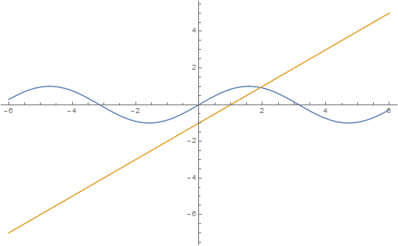
Here's a short example adapted from The Student's Introduction to Mathematica. What is instructive is they Plot the two components of the equation separately. Analyzing and plotting each term separately is essential to understanding the equation as a whole.

Use TraditionalForm to put an expression in traditional math format:

Sin@x==x-1//TraditionalForm
sin(x) = x – 1

With Plot we visualize the two terms of the equation as separate functions and their intersection, indicating where they zero each other out near x = 2. Giving Plot the two terms in a List says 'Plot y = sin(x) and y = x - 1 together.' The first function is blue, the second, yellow.

Plot[{Sin@x, x - 1}, {x, -6, 6}]


Since we have flushed out a root, we can use FindRoot to precisely locate it, supplying FindRoot with a guess that it's near x = 2. Giving FindRoot a single coordinate causes it to use the Newton-Raphson method, while giving it two coordinates causes it to use a secant method.

soln1=FindRoot[Sin@x==x-1,{x,2}]
{x->1.93456}

Always verify the solution.

Sin@x==x-1/.soln1

True


Thursday, June 4, 2015

Examples of Different Programming Styles with Timing

This comparison of different programming styles is adapted from Roman Maeder's in his Programming in Mathematica course. Here is a List of expressions to square, including different types on numbers and an undefined symbol.

alist={a,1.1,2+3I,4,573297329847};


Functional Style


Here is the shortest solution, which works due to the function Attribute, Listable, of Power that maps Power over a List. You can add Listable to your own functions to achieve the same simplicity.

squareListListable@list_List:=list^2

squareListListable@alist
{a^2,1.21,-5+12 I,16,328669828409699917043409}

As Maeder says, it really cannot get much simpler than that. Here are two more functional-style solution. These are also compact. The first uses Table, a very powerful function that leads us to not deconstruct lists (arrays) but to think of applying a function to them as a whole. The simple squaring of each List item could be replaced with a function of arbitrary complexity.

squareFunctional@list_List:=Table[i^2,{i,list}]

Beginners are often unaware of Table's ability to iterate directly over List items, as above, without this unnecessary clutter. However, see the Timing analysis below for a surprise.

squareFunctionalWithIterator@list_List:=Table[list[[i]]^2,{i,Length@list}]

This third functional example uses Map, another powerful function that, along with Listable and Table, replaces the Do loop. A pure Function expresses the squaring operation concisely.

squareListMapped@list_List:=Map[#^2&,list]


Rule-Based Style


Programming with replacement rules is the way Mathematica itself works — Every Change is a Transformation — and rule-based functions are often very concise and easy to understand. I prefer rule-based functions over other styles.

squareRuleBasedShorter@list_List:=list/.{first___,x_,rest___}->{first,x^2,rest}


Recursive Style


Here is a recursive rule-based approach — the function calls itself and keeps marching down a 'rest' of List that keeps getting smaller. Note that flattening deeply nested Lists is a very fast operation (Log@n) whose timing you rarely need to worry about. However this recursive approach is only practical for small examples.

squareRuleRecursive@list_List:=list/.{x_,rest___}:>{x^2,squareRuleRecursive@{rest}}//Flatten

Procedural Style


While I really think which style to use is a personal decision ('de gustibus non est disputandum'), this procedural solution does seem cumbersome and old-fashioned compared to the functional and rule-based ones. But sometimes procedural functions are easier and faster to write than laboring to find more concise functional or rule-based ones.

squareProcedural@list_List:=Module[{array1={},squaresList,
listLength=Length@list},
Do[array1=Prepend[array1,0],{i,listLength}];
Do[array1[[i]]=list[[i]]^2,{i,listLength}];
Return@array1
]

Maeder cheats a bit, using Table to initialize his array, which speeds up his function considerably as you'll see in the Timing analysis.

squareProceduralMaeder@list_List:=Module[
{squaresArray,
listLength=Length@list},
(*initialize the array*)
squaresArray=Table[0,{listLength}];
Do[squaresArray[[i]]=list[[i]]^2,{i,listLength}];
Return@squaresArray
]


Timing Analysis


aLongList=Range[10^6];

The Listable function is the clear winner.

Timing[squareListListable@aLongList;]
{0.,Null}

Let's push it harder to see more of its speed advantage. It appears to be 10 times faster than its competitors below.

Timing[squareListListable@Range[10^7];]
{0.015600,Null}

Timing[squareFunctional@aLongList;]
{0.031200,Null}

Here's the surprise I mentioned. Not sure why, but using the iterator is exactly twice as fast than 'directly' iterating over List items. I'd only worry about this for functions needing optimization though.

Timing[squareFunctionalWithIterator@aLongList;]
{0.015600,Null}

Timing[squareListMapped@aLongList;]
{0.015600,Null}

It surprise me that the rule-based approach is relatively slow.

Timing[squareRuleBased@aLongList;]
{0.062400,Null}

Both the recursive and procedural approaches are very slow.

Timing[squareRuleRecursive@aLongList;]
During evaluation of In[186]:= $RecursionLimit::reclim: Recursion depth of 1024 exceeded. >>
Out[186]= {9.188459,Null}

Timing[squareProcedural@aLongList;]
$Aborted

Timing[squareProceduralMaeder@aLongList;]

{2.012413,Null}

Wednesday, June 3, 2015

Two Ways to Add Line Numbers to a Table

Often we'd like to add line numbers to a table of data. Here's a simple method using the formula for distance traveled in meters by a falling body near the earth's surface (0.5 x 9.8 m/s2).

Using Table with Iterator

It is easy to see that the lone iterator "i" simply supplies the line numbers, indicating 1 to 20 seconds, for TableForm.

Table[{i,4.9 i^2},{i,20}]//TableForm


Here's a fancier version with headings. The first "None" in TableHeadings is for row labels, which we don't need since the Table iterator provided them, while the second set of values are the column headings. TableForm doesn't provide for a title, but we can add one with Labeled. A "\n" creates a line break and we need Style to center the title.


Table[{i,4.9 i^2},{i,20}]//TableForm[#,TableHeadings->{None,{"Seconds","Meters"}}]&//Labeled[#,"Distance Traveled in 20 Seconds\nof Free Fall Near the Earth's Surface\n",Top]&//Style[#,TextAlignment->Center]&


Using MapIndexed

Here the formula for distance in feet is expressed in pure Function shorthand, which is then mapped onto the integers from 1 to 20 generated by Range, representing 20 seconds of free fall from v0 = 0. A pure Function is the fast way to write a one-off function that you don't intend to re-use.

MapIndexed adds the index to the expression as a suffix, so we need to Map Reverse on to each data item that will be a row in the table.

MapIndexed[{16#^2,#2}&,Range@2]

Out[53]= {{16,{1}},{64,{2}}}

Last we apply TableForm.

MapIndexed[{4.9 #^2, #2} &, Range@20] // Reverse /@ # & // TableForm


Monday, June 1, 2015

Use Packages to Extend Mathematica with Your Own Functions

The framework for extending Mathematica with user-created programs, like library functions in many programming languages, is provided by Packages. 

Generally use Needs to load Packages, not Get. Needs checks to see if a Package is already loaded. But use Get when developing a Package since in that case you want to overwrite the old Package.

Here are the essentials of what you need to know to create Packages of your own. This table steps through an example of a Package. See the line-by-line comments below the table for an explanation of what’s going on in each step.

Line/Comment #
Command
$Context
$ContextPath
1
Times[4, Pi, Power[2, 2]]
Global`
{Global`, System`}
2
area@radius_:= 4*Pi*r^2
Global`
{Global`, System`}
3
BeginPackage@“MyFunctions`”]
MyFunctions`
{MyFunctions` , System`}
4
sphereArea::usage=” sphereArea @radius calculates the area of a sphere of radius r.”
MyFunctions`
{MyFunctions `, System`}
5
Begin@” MyFunctions `Private`”
MyFunctions `Private`
{MyFunctions `, System`}
6
sphereArea@radius_:= 4*Pi*r^2
MyFunctions `Private`
{MyFunctions `, System`}
7
circumference@radius_:= 2*Pi*r
MyFunctions `Private`
{MyFunctions `, System`}
8
End[]
MyFunctions`
{MyFunctions `, System`}
9
EndPackage[]
Global`
{MyFunctions `, Global`,System`}

Comment by Line Number

  1. A Mathematica session begins in the Global` Context. All built-in commands reside in the System` Context, which is always on the Context search path stored in $ContextPath) so they can be found no matter what Context you are in. This is the FullForm of a calculation for the surface area of a sphere with radius = 2 using built-in commands Times, Power, and constant Pi.
  2. All user-defined symbols, including function names and definitions, reside in the Global` Context and are globally visible, along with built-in commands in the System` Context, unless the user changes the Context. This function is a one-off for calculating the surface area of a sphere.
  3. BeginPackage changes the current Context to that of the Package it names, removes all Contexts except System (so built-in commands are accessible) from $ContextPath, and adds the Package name to $ContextPath. BeginPackage removes all Contexts, especially the Global` Context, from $ContextPath so that no globally-visible, previously-defined symbols can foul you up while you develop your Package. Thus you can use the same names while fooling around in Global` that you may end up using in the Package.
  4. Usage messages not only return their content when queried with Information@symbol (“?symbol”) but expose the function name for use outside the Package.
  5. Symbols in a Private` Context are not visible on the Context search path. But since a usage message declared sphereArea in the public Package Context, it will be found when used in any Context. I suspect while we always see short ‘nicknames’ for symbols, which are the last Context path element, Mathematica always sees the full Context path names, thus is omniscient and ambiguity between identical names is resolved.
  6. A function for calculating the surface area of a sphere, like the one-off one in Global`, is more formally defined for repeated use in the future, corresponding to the usage message placed in the public area of the Package (see #4). This definition, in the Private area of the Package, is invisible while any definition in the usage message is visible (e.g. using “?sphereArea”).
  7. A private function calculating the circumference of a circle is defined for use within the Package by other functions but not for public export. It cannot be seen outside the Package (unless its full Context path is entered).
  8. End[] ) - no argument is used - is the command used to exit a Context, in this case, “MyFunctions`Private`”, which removes the most recent Context entered in $ContextPath and returns us to the previous Context, “MyFunctions`”.
  9. EndPackage[]- no argument is used - exits the Package and adds any other Contexts, in this case Global`, to the Context search path. 

Further guidance:

For consistency, make the name of a Package file the same as Context it uses (e.g. here, "MyFunctions.m"). Put the Package file in a directory in $Path (the directory List searched by Mathematica), such as that specified by $UserBaseDirectory, which is the location Mathematica provides for user Packages, or add your Package file’s directory to $Path with PrependTo.

Test your Package with typical parameter values for which it was designed, but also incorrect datatypes and values outside the range for which it was designed,
You can Protect a symbol from alteration by a user with SetAttributes[aSymbol, Protected].

You can Protect a symbol’s definition from being read by a user with SetAttributes[aSymbol, ReadProtected]

Whether in a Notebook or Package (.m) file, cells that you want to be automatically evaluated must be Initialization cells (Cell => Cell Properties => Initialization Cell).

Sources
Programming in Mathematica Course by Roman Maeder, Wolfram Research, Inc.
David Wagner, Power Programming with Mathematica: The Kernel  (New York: McGraw-Hill, 1996. out of print).
StackExchange discussion here.